Calculating future returns in Python
Calculating the potential future value of Bitcoin Investment
The year 2017 was a great year for cryptocurrencies and in particular for the crypto leader Bitcoin. Many people called crypotcurrencies the future of money, but so far 2018 has been lousy. The crypto currency advocates argue that the value of will increase in the future. We have seen many claims, from $50000 to $1000000 per bitcoin. We take no sides and the Market will decide the future. For this example we want to demonstrate how much one can make in Bitcoin, if the predictions are correct. Our focus is not on making predictions, but on learning to perform future value calculations in Python.
Since the end 2010 Bitcoin prices have gone up from about $0.05 to about $6500 today. That is a 320% increase per year. We don’t believe that it will continue at that pace in the future, but let’s say it grows at 1/10th of that or 35% per year (still a big leap of faith and hard to replicate).
Since this is a speculation, we will not risk too much on this and speculate only $1000 on this idea. How much would a $1000 investment(its really a speculation) in Bitcoin be after 30 years at 35% per year?
First lets load our libraries as usual.
import numpy as np
import pandas as pd
Next we will present the entire code at once and then go through it.
bitcoin_speculation = 1000 # Speculating $1000 on bitcoin
returns = 0.35 # Assuming 35% returns
# Creating an empty table
fv_table = np.zeros((30,4))
fv_table = pd.DataFrame(fv_table)
fv_table.columns = ['Year', 'beg_val', 'ret', 'end_val']
fv_table['Year'] = np.arange(1,31)
# Calculating the first row values
fv_table.iloc[0,1] = bitcoin_speculation
fv_table.iloc[0,2] = returns * bitcoin_speculation
fv_table.iloc[0,3] = fv_table.iloc[0,1] + fv_table.iloc[0,2]
# For loop
for i in range(1,30):
    fv_table.iloc[i,1] = fv_table.iloc[(i-1),3]
    fv_table.iloc[i,2] = fv_table.iloc[i,1] * returns
    fv_table.iloc[i,3] = fv_table.iloc[i,1] + fv_table.iloc[i,2]

print(fv_table.tail().round(2))
## Year beg_val ret end_val
## 25 26 1812776.29 634471.70 2447247.99
## 26 27 2447247.99 856536.80 3303784.79
## 27 28 3303784.79 1156324.68 4460109.47
## 28 29 4460109.47 1561038.31 6021147.78
## 29 30 6021147.78 2107401.72 8128549.50So we can see that at 35% per year an investment can grow to $8.128 million in 30 years.
Now lets go through this together.
First we setup our variable and create the empty table using the np.zeros() functions and then convert it into a pandas dataframe.
bitcoin_speculation = 1000 # Speculating $1000 on bitcoin
returns = 0.35 # Assuming 35% returns
# Creating an empty table
fv_table = np.zeros((30,4))
fv_table = pd.DataFrame(fv_table)
fv_table.columns = ['Year', 'beg_val', 'ret', 'end_val']
fv_table['Year'] = np.arange(1,31)
Next we need to calculate the first row manually. We need to be careful with Python indexing sine it starts at 0.
# Calculating the first row values
fv_table.iloc[0,1] = bitcoin_speculation
fv_table.iloc[0,2] = returns * bitcoin_speculation
fv_table.iloc[0,3] = fv_table.iloc[0,1] + fv_table.iloc[0,2]
print(fv_table.head().round(2))
## Year beg_val ret end_val
## 0 1 1000.0 350.0 1350.0
## 1 2 0.0 0.0 0.0
## 2 3 0.0 0.0 0.0
## 3 4 0.0 0.0 0.0
## 4 5 0.0 0.0 0.0We can see that we have changed the value of the first row and next we apply the same formula to all the columns using the for loop.
for i in range(1,30):
    fv_table.iloc[i,1] = fv_table.iloc[(i-1),3]
    fv_table.iloc[i,2] = fv_table.iloc[i,1] * returns
    fv_table.iloc[i,3] = fv_table.iloc[i,1] + fv_table.iloc[i,2]
# Showing only the tail of the table
print(fv_table.round(2))
## Year beg_val ret end_val
## 0 1 1000.00 350.00 1350.00
## 1 2 1350.00 472.50 1822.50
## 2 3 1822.50 637.88 2460.38
## 3 4 2460.38 861.13 3321.51
## 4 5 3321.51 1162.53 4484.03
## 5 6 4484.03 1569.41 6053.45
## 6 7 6053.45 2118.71 8172.15
## 7 8 8172.15 2860.25 11032.40
## 8 9 11032.40 3861.34 14893.75
## 9 10 14893.75 5212.81 20106.56
## 10 11 20106.56 7037.29 27143.85
## 11 12 27143.85 9500.35 36644.20
## 12 13 36644.20 12825.47 49469.67
## 13 14 49469.67 17314.38 66784.05
## 14 15 66784.05 23374.42 90158.47
## 15 16 90158.47 31555.46 121713.93
## 16 17 121713.93 42599.88 164313.81
## 17 18 164313.81 57509.83 221823.64
## 18 19 221823.64 77638.27 299461.92
## 19 20 299461.92 104811.67 404273.59
## 20 21 404273.59 141495.76 545769.35
## 21 22 545769.35 191019.27 736788.62
## 22 23 736788.62 257876.02 994664.63
## 23 24 994664.63 348132.62 1342797.25
## 24 25 1342797.25 469979.04 1812776.29
## 25 26 1812776.29 634471.70 2447247.99
## 26 27 2447247.99 856536.80 3303784.79
## 27 28 3303784.79 1156324.68 4460109.47
## 28 29 4460109.47 1561038.31 6021147.78
## 29 30 6021147.78 2107401.72 8128549.50As we can see from the table our $1000 investment would grow to approximately $8.13 million in 30 years. When you think of saving $1000/year, its not that difficult. If a person saves $3 per day for an entire year, he/she would have $1000. But as mentioned above, growing at 35% per year for 30 years is incredibly hard. So it may never reach that price. We are curious to see how Bitcoin story unfolds.
Calculating the future value of regular annual deposits
In the last example we saw the hypothetical growth of Bitcoin and how an investment grows at 35% per year. It is quite lofty to grow at 35% per year and is highest form of speculation and may not be suitable for all. So one should be careful and not bet a huge amount on such activities.
So what about the regular savers. How can we calculate their future values and whether its enough for their retirement? Does it matter when you start saving? We will answer these questions in the next example.
Consider an example of Tom and Jerry. They are the same age, but both have different personalities. Tom believes in securing his future and works hard towards it, Jerry believes in living in the moment and only start saving after securing a higher paying job. At the end of every month Tom strives to save 10% of his salary, Jerry always finds himself without any money left.
Lets assume they are both 20 and starting their first job. They make $3000 per month. They wish to retire in 50 years. Tom decides to save and invest for first 20 years age 20 to 40 and then no savings after that. Jerry on the other hand also decides to save and invest 10% of his salary for 20 years but from age 50 to 70. For simplicity we will assume their salary stays the same and ignore taxes. We also assume they make 7.5% on their investments, which close to the historical returns on US stock market over the long term.
How will they do?
What do we know.
- Yearly salary $36000 (3000 per month)
- Yearly deposit $3600
- Stock Returns 7.5%
- Both save for the same duration 20 year, but their timing is different.
- Tom saves from age 20 to 40
- Jerry save from age 50 to 70
- They both will retire at age 70
If you have followed this calculations in R, this is similar. The code is broken down into three parts. First part calculates Tom’s table, the second part calculates Jerry’s table and the third part combines the two tables.
# Jerry's Table
returns = 0.075
annual_deposit = 3600
# Creating the empty table
fv_table = np.zeros((50,5))
fv_table = pd.DataFrame(fv_table)
fv_table.columns = ['Year', 'beg_val', 'deposit', 'ret', 'end_val']
fv_table['Year'] = np.arange(1,51)
# Calculating the first row values
fv_table.iloc[0,2] = annual_deposit
fv_table.iloc[0,3] = annual_deposit * returns
fv_table.iloc[0,4] = fv_table.iloc[0,3] + fv_table.iloc[0,2]
# Running the for loop for first phase
for i in range(1,20):
    fv_table.iloc[i,1] = fv_table.iloc[(i-1),4]
    fv_table.iloc[i,2] = annual_deposit
    fv_table.iloc[i,3] = (fv_table.iloc[i,1] + fv_table.iloc[i,2]) * returns
    fv_table.iloc[i,4] = (fv_table.iloc[i,1] + fv_table.iloc[i,2]) \
    * returns + annual_deposit + fv_table.iloc[i,1]


# Running the for loop for the second phase
for i in range(20,50):
    fv_table.iloc[i,1] = fv_table.iloc[(i-1),4]
    fv_table.iloc[i,3] = (fv_table.iloc[i,1] + fv_table.iloc[i,2]) * returns
    fv_table.iloc[i,4] = (fv_table.iloc[i,1] + fv_table.iloc[i,2]) \
    * returns + fv_table.iloc[i,1]

# Saving Table for Tom
fv_table_tom = fv_table
# ------------------------------------------------------------------------------------
# Setup variables
returns = 0.075
annual_deposit = 3600
# Create empty table
fv_table = np.zeros((21,5))
fv_table = pd.DataFrame(fv_table)
fv_table.columns = ['Year', 'beg_val', 'deposit', 'ret', 'end_val']
fv_table['Year'] = np.arange(1,22)
fv_table['Year'] = np.arange(30,51)
# Computer the first row values
fv_table.iloc[0,2] = annual_deposit
fv_table.iloc[0,3] = annual_deposit * returns
fv_table.iloc[0,4] = fv_table.iloc[0,3] + fv_table.iloc[0,2]
# Run the for loop
for i in range(1,21):
    fv_table.iloc[i,1] = fv_table.iloc[(i-1),4]
    fv_table.iloc[i,2] = annual_deposit
    fv_table.iloc[i,3] = (fv_table.iloc[i,1] + fv_table.iloc[i,2]) * returns
    fv_table.iloc[i,4] = (fv_table.iloc[i,1] + fv_table.iloc[i,2]) \
    * returns + annual_deposit + fv_table.iloc[i,1]

fv_table_jerry = fv_table
# ------------------------------------------------------------------------------------
# join the tables
fv_table_both = pd.merge(fv_table_tom,fv_table_jerry, on = "Year", how = "outer")
# Rename the columns
fv_table_both.columns = ["Year", "Tom's initial value", "Tom's Deposit",\
                         "Tom's Interest", "Tom's Ending value", \
                         "Jerry's initial value", "Jerry's Deposit", \
                         "Jerry's Interest", "Jerry's Ending value"]


fv_table_both = fv_table_both.fillna(0).round(2)
# Showing only 3 columns
print(fv_table_both[["Year", "Tom's Ending value", "Jerry's Ending value"]])
## Year Tom's Ending value Jerry's Ending value
## 0 1 3870.00 0.00
## 1 2 8030.25 0.00
## 2 3 12502.52 0.00
## 3 4 17310.21 0.00
## 4 5 22478.47 0.00
## 5 6 28034.36 0.00
## 6 7 34006.94 0.00
## 7 8 40427.46 0.00
## 8 9 47329.51 0.00
## 9 10 54749.23 0.00
## 10 11 62725.42 0.00
## 11 12 71299.83 0.00
## 12 13 80517.31 0.00
## 13 14 90426.11 0.00
## 14 15 101078.07 0.00
## 15 16 112528.93 0.00
## 16 17 124838.60 0.00
## 17 18 138071.49 0.00
## 18 19 152296.85 0.00
## 19 20 167589.12 0.00
## 20 21 180158.30 0.00
## 21 22 193670.17 0.00
## 22 23 208195.44 0.00
## 23 24 223810.09 0.00
## 24 25 240595.85 0.00
## 25 26 258640.54 0.00
## 26 27 278038.58 0.00
## 27 28 298891.47 0.00
## 28 29 321308.33 0.00
## 29 30 345406.46 3870.00
## 30 31 371311.94 8030.25
## 31 32 399160.34 12502.52
## 32 33 429097.36 17310.21
## 33 34 461279.67 22478.47
## 34 35 495875.64 28034.36
## 35 36 533066.32 34006.94
## 36 37 573046.29 40427.46
## 37 38 616024.76 47329.51
## 38 39 662226.62 54749.23
## 39 40 711893.61 62725.42
## 40 41 765285.64 71299.83
## 41 42 822682.06 80517.31
## 42 43 884383.21 90426.11
## 43 44 950711.95 101078.07
## 44 45 1022015.35 112528.93
## 45 46 1098666.50 124838.60
## 46 47 1181066.49 138071.49
## 47 48 1269646.47 152296.85
## 48 49 1364869.96 167589.12
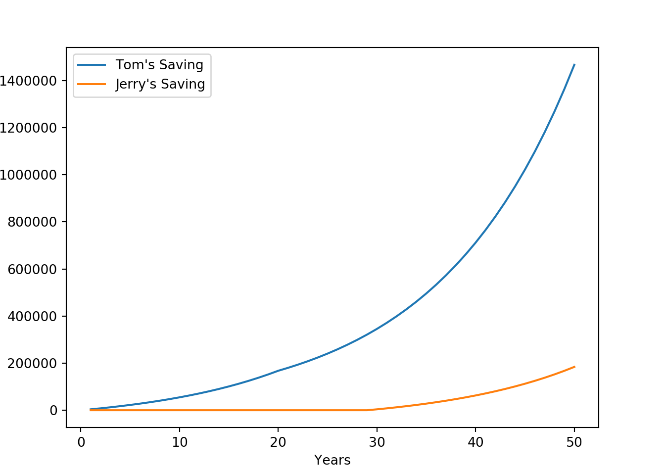
## 49 50 1467235.21 184028.30We can also plot the savings chart for both Tom and Jerry.
import matplotlib.pyplot as plt
fig = plt.figure()
ax1 = plt.axes([0.1,0.1,0.8,0.8])
ax1.plot(fv_table_both['Year'], fv_table_both['''Tom's Ending value'''], label = "Tom's Saving")
ax1.plot(fv_table_both['Year'], fv_table_both['''Jerry's Ending value'''], label = "Jerry's Saving")
ax1.set_xlabel("Years")
ax1.set_ylabel("Saving growth")
plt.legend(loc = "best")
plt.show()