How to download stock prices in Python
Getting stock prices from Yahoo Finance
One of the most important tasks in financial markets is to analyze historical returns on various investments. To perform this analysis we need historical data for the assets. There are many data providers, some are free most are paid. In this chapter we will use the data from Yahoo’s finance website. Since Yahoo was bought by Verizon, there have been several changes with their API. They may decide to stop providing stock prices in the future. So the method discussed on this article may not work in the future.
Python module for downloading price data
Python has a module called pandas-datareader which is used for downloading financial data from yahoo. You can install it by typing the command pip install pandas-datareader in your terminal/command prompt (update as of 2019 this is no longer true, use the fix-yahoo-finance module).
Let us load the modules/libraries
import pandas as pd
import pandas_datareader as web
import numpy as np
import matplotlib.pyplot as plt
We will download Apple stock’s price first.
aapl = web.get_data_yahoo("AAPL",
start = "2017-01-01",
end = "2018-03-01")
Lets look at the head of the data.
print(aapl.head())## High Low ... Volume Adj Close
## Date ...
## 2017-01-03 116.330002 114.760002 ... 28781900.0 111.709831
## 2017-01-04 116.510002 115.750000 ... 21118100.0 111.584778
## 2017-01-05 116.860001 115.809998 ... 22193600.0 112.152229
## 2017-01-06 118.160004 116.470001 ... 31751900.0 113.402542
## 2017-01-09 119.430000 117.940002 ... 33561900.0 114.441246
##
## [5 rows x 6 columns]We can plot the data for Apple.
aapl["Adj Close"].plot()
plt.xlabel("Date")
plt.ylabel("Adjusted Price")
plt.title("Apple price data")
plt.show()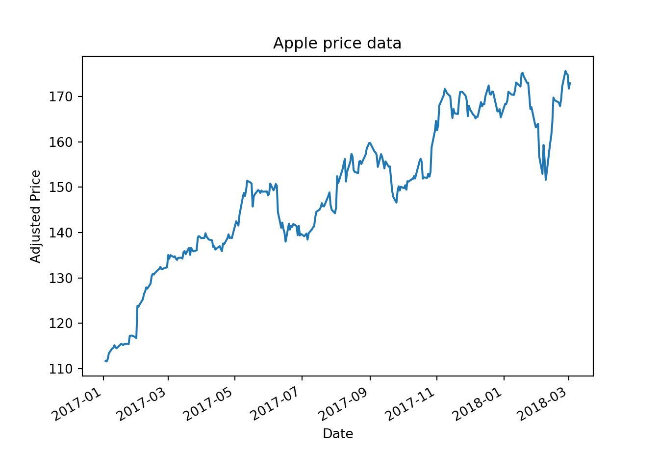
We can also download the data for multiple stocks using the below command.
tickers = ["AAPL", "MSFT", "AMZN", "K", "O"]
prices = web.get_data_yahoo(tickers,
start = "2017-01-01",
end = "2017-01-15")
We can look at the head of the data.
print(prices.head())## Attributes High ... Adj Close
## Symbols AAPL AMZN ... MSFT O
## Date ...
## 2017-01-03 116.330002 758.760010 ... 59.694695 51.610588
## 2017-01-04 116.510002 759.679993 ... 59.427597 52.382626
## 2017-01-05 116.860001 782.400024 ... 59.427597 53.792084
## 2017-01-06 118.160004 799.440002 ... 59.942703 53.720253
## 2017-01-09 119.430000 801.770020 ... 59.751923 53.325245
##
## [5 rows x 30 columns]As we can see that all the stock prices have been merged in one table. We can also just look at the adjusted prices.
prices["Adj Close"].head()Next we can plot prices of the stocks.
prices["Adj Close"].plot()
plt.xlabel("Date")
plt.ylabel("Adjusted Price")
plt.title("All stocks price data")
plt.show()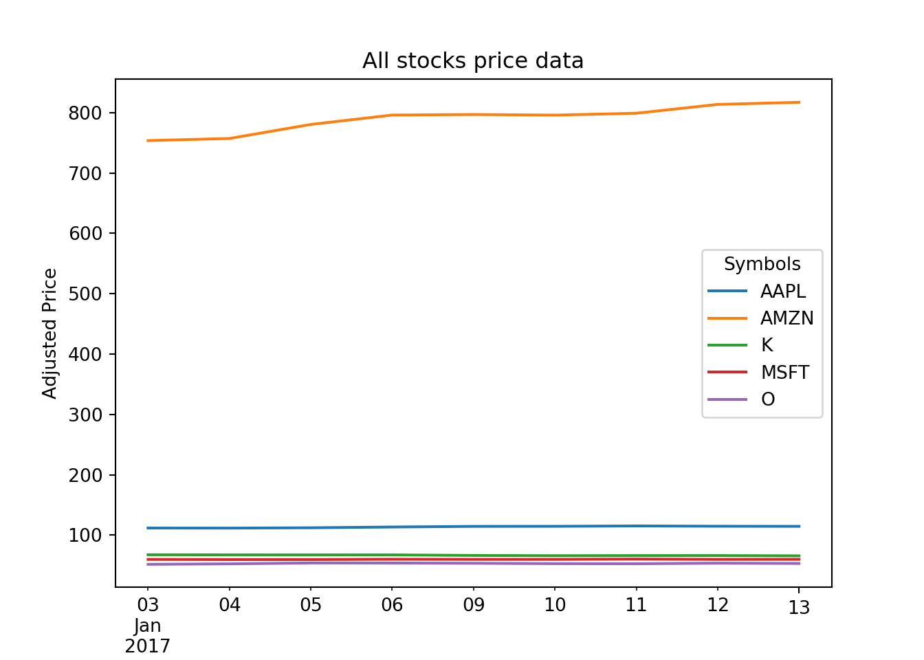
This chart has the same problem as before as the there is wide variation in the price data. To solve this problem we will have to calculate the cumulative returns and plot that data. We will discuss that in the next post.