Download Fama French Data

Because we will be downloading and cleaning our Fama French data many times, we will automate this step and build a function. This way we won’t have to repeat the steps for our analysis each time we analyze a new fund.

So lets build our function. The steps are all similar to what we did in the past. We are just wrapping those steps in a function.

# Automate Getting Fama French data from the website

get_fama_french <- function() {
  
  #This is the URL for the website
  
  ff_url <- "https://mba.tuck.dartmouth.edu/pages/faculty/ken.french/ftp/F-F_Research_Data_Factors_CSV.zip"
  
  # Create a temp file to store the data
  
  temp_file <- tempfile()
  
  # Download the data
  
  download.file(ff_url, temp_file,quiet = TRUE)
  
  # Unzip & Read the data
  ff_data_raw <- read_csv(unzip(temp_file), skip = 3)
  
  # This step is to delete the extra data that is not needed 
  # We are getting the row index where the data ends
  
  ff_row <- which(is.na(ff_data_raw$SMB))
  ff_row <- ff_row[1]
  
  # Selecting only the rows we need for our analysis
  
  ff_data_raw <- ff_data_raw[c(1:(ff_row - 1)),]
  
  # Changing the Column names
  
  colnames(ff_data_raw) <- paste(c('date', "mkt_excess", "smb", "hml", "rf"))
  
  # Formatting the date column
  # We want the end of the month dates
  ff_data_raw <- ff_data_raw %>%
    mutate(date = ymd(parse_date(date, format = "%Y%m"))) %>%
    mutate(date = date + months(1)) %>% # Add one month
    mutate(date = rollback(date)) # change it back to end of the month
  
  # Finally converting the data from percent to decimal
  
  ff_data_raw <- ff_data_raw %>%
    mutate_at(vars(-date), function(x) x/100)
  
  return(ff_data_raw)
  
}

Now that we have built the function to get Fama French data automatically, lets test it.

ff_data <- get_fama_french()

head(ff_data)

## # A tibble: 6 x 5
##   date       mkt_excess     smb      hml     rf
##   <date>          <dbl>   <dbl>    <dbl>  <dbl>
## 1 1926-07-31     0.0296 -0.023  -0.0287  0.0022
## 2 1926-08-31     0.0264 -0.0140  0.0419  0.0025
## 3 1926-09-30     0.0036 -0.0132  0.0001  0.0023
## 4 1926-10-31    -0.0324  0.0004  0.0051  0.0032
## 5 1926-11-30     0.0253 -0.002  -0.00350 0.0031
## 6 1926-12-31     0.0262 -0.0004 -0.0002  0.0028

tail(ff_data)

## # A tibble: 6 x 5
##   date       mkt_excess     smb     hml     rf
##   <date>          <dbl>   <dbl>   <dbl>  <dbl>
## 1 2018-12-31    -0.0955 -0.0258 -0.0151 0.0019
## 2 2019-01-31     0.0841  0.0302 -0.006  0.0021
## 3 2019-02-28     0.034   0.0202 -0.0284 0.0018
## 4 2019-03-31     0.011  -0.0315 -0.0407 0.0019
## 5 2019-04-30     0.0396 -0.017   0.0198 0.0021
## 6 2019-05-31    -0.0694 -0.0125 -0.0238 0.0021

We can see that data has been downloaded properly and just for sanity check we should plot it.

ff_data %>%
  gather(mkt_excess:rf, key = name, value = val) %>%
  group_by(name) %>%
  mutate(ret = cumprod(1 + val)) %>%
  ggplot(aes(x = date, y = ret, color = name)) +
  geom_line() +
  scale_y_log10()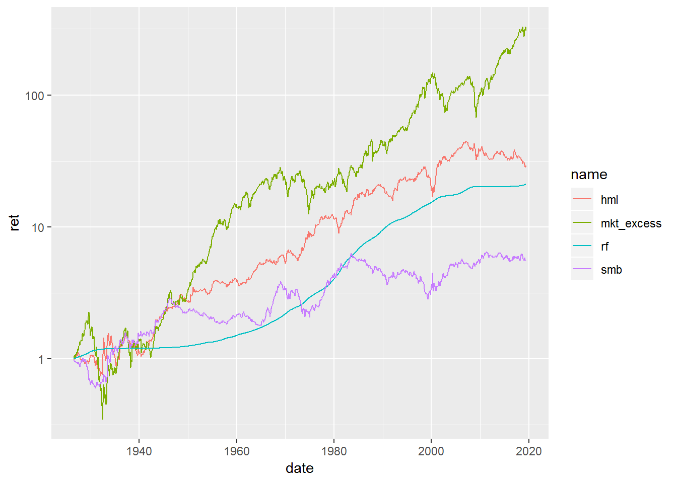

The plot confirms that the data has been downloaded correctly. We see no spikes or dips in our time series.

Download the Mutual Fund Data

Next lets choose a mutual fund to analyze. For this exercise we wanted to choose an active mutual fund that has been managed for a long time. The size of the mutual fund also needs to be large. So we selected the Fidelity Contrafund Fund (FCNTX). The fund has data going as far back as 1980.

So lets download the data for the fund. Again we want to automate the process of downloading the price data for funds, this will accelerate our process and we will spend more time in analyzing the result versus downloading the data. We will build another function to do that.

# Type the ticker name

ticker <- "FCNTX"

# So this function requires the ticker, start and end date
# as arguments

get_price_data <- function(ticker, start, end) {
  
  price_data <- tq_get(ticker,
                       from = start,
                       to = end,
                       get = 'stock.prices')
  
  return(price_data)
  
}

Now lets test our function.

# Type the ticker name

ticker <- "FCNTX"

# Start date
start <- "1980-01-01"

# End Date since we have FF data only till May

end <- "2019-05-31"

# Download the price

price_data <- get_price_data(ticker, start, end)

Again lets plot it to make sure the data has been downloaded correctly.

price_data %>%
  ggplot2::aes(date, adjusted) +
  geom_line()

## NULL

head(price_data)

## # A tibble: 6 x 7
##   date        open  high   low close volume adjusted
##   <date>     <dbl> <dbl> <dbl> <dbl>  <dbl>    <dbl>
## 1 1980-01-02  1.14  1.14  1.14  1.14      0    0.169
## 2 1980-01-03  1.12  1.12  1.12  1.12      0    0.167
## 3 1980-01-04  1.14  1.14  1.14  1.14      0    0.170
## 4 1980-01-07  1.14  1.14  1.14  1.14      0    0.169
## 5 1980-01-08  1.17  1.17  1.17  1.17      0    0.174
## 6 1980-01-09  1.17  1.17  1.17  1.17      0    0.174

tail(price_data)

## # A tibble: 6 x 7
##   date        open  high   low close volume adjusted
##   <date>     <dbl> <dbl> <dbl> <dbl>  <dbl>    <dbl>
## 1 2019-05-22  12.8  12.8  12.8  12.8      0     12.8
## 2 2019-05-23  12.6  12.6  12.6  12.6      0     12.6
## 3 2019-05-24  12.6  12.6  12.6  12.6      0     12.6
## 4 2019-05-28  12.6  12.6  12.6  12.6      0     12.6
## 5 2019-05-29  12.5  12.5  12.5  12.5      0     12.5
## 6 2019-05-30  12.5  12.5  12.5  12.5      0     12.5

Calculate the Returns Data

Next we will build another function that calculates the returns for our fund. Now we could have easily combined the function to download the price and calculate the returns together. But this is not a good programming practice. In general we want our functions (automation) to do one thing only. This makes it very easy to debug our programs.

So lets calculate the returns

# Automating the returns calculation

# We need to provide the price data table
# And the period, by default is monthly
# Since FF data is monthly

get_return_data <- function(closing_price, period = "monthly") {
  
  # This step check to see if there are more than 1 tickers
  
  is_symbol <- "symbol" %in% colnames(closing_price)
  
  # If we have more tickers then we will use groupby()
  if (is_symbol == TRUE) {
    
    ret_data <- closing_price %>%
      group_by(symbol) %>%
      tq_transmute(select = adjusted,
                   mutate_fun = periodReturn,
                   period = period,
                   col_rename = 'returns')
    
    return(ret_data)
    
    # If we have only 1 tickers, we don't use groupby()
  } else {
    
    ret_data <- closing_price %>%
      tq_transmute(select = adjusted,
                   mutate_fun = periodReturn,
                   period = period,
                   col_rename = 'returns')
    
    return(ret_data)
    
  }
  
}

Lets use our function to calculate the returns

ret_data <- get_return_data(price_data,"monthly")

head(ret_data)

## # A tibble: 6 x 2
##   date        returns
##   <date>        <dbl>
## 1 1980-01-31 -0.00968
## 2 1980-02-29 -0.0169 
## 3 1980-03-31 -0.0894 
## 4 1980-04-30  0.0179 
## 5 1980-05-30  0.0789 
## 6 1980-06-30  0.0117

tail(ret_data)

## # A tibble: 6 x 2
##   date       returns
##   <date>       <dbl>
## 1 2018-12-31 -0.0804
## 2 2019-01-31  0.0945
## 3 2019-02-28  0.0240
## 4 2019-03-29  0.0221
## 5 2019-04-30  0.0488
## 6 2019-05-30 -0.0442

Combine the data and run Regression

Once again we will build a function to combine the data and then another function that runs the multiple regression model on our data.

# We want the data to match the last day of our FF date

last_month_ff <- ff_data %>%
  select(date) %>%
  slice(nrow(ff_data)) %>%
  .[[1]]

# Join the portfolio data with FF data

join_data <- function(ret_data, ff_data) {
  
  
  joined_data <- ret_data %>%
    filter(date <= last_month_ff) %>%
    mutate(date = rollback(date, roll_to_first = TRUE)) %>%
    mutate(date = date + months(1)) %>%
    mutate(date = rollback(date)) %>%
    left_join(ff_data,by = 'date') %>%
    mutate(port_excess = returns - rf)
    
  
  return(joined_data)

}

Now lets see if the data was joined correctly.

ff_data <- join_data(ret_data,ff_data)

head(ff_data)

## # A tibble: 6 x 7
##   date        returns mkt_excess     smb     hml      rf port_excess
##   <date>        <dbl>      <dbl>   <dbl>   <dbl>   <dbl>       <dbl>
## 1 1980-01-31 -0.00968     0.0551  0.0165  0.018  0.008      -0.0177 
## 2 1980-02-29 -0.0169     -0.0122 -0.0182  0.0062 0.0089     -0.0258 
## 3 1980-03-31 -0.0894     -0.129  -0.0664 -0.0106 0.0121     -0.102  
## 4 1980-04-30  0.0179      0.0397  0.0097  0.0106 0.0126      0.00526
## 5 1980-05-31  0.0789      0.0526  0.0216  0.0039 0.0081      0.0708 
## 6 1980-06-30  0.0117      0.0306  0.0167 -0.0089 0.00610     0.00564

tail(ff_data)

## # A tibble: 6 x 7
##   date       returns mkt_excess     smb     hml     rf port_excess
##   <date>       <dbl>      <dbl>   <dbl>   <dbl>  <dbl>       <dbl>
## 1 2018-12-31 -0.0804    -0.0955 -0.0258 -0.0151 0.0019     -0.0823
## 2 2019-01-31  0.0945     0.0841  0.0302 -0.006  0.0021      0.0924
## 3 2019-02-28  0.0240     0.034   0.0202 -0.0284 0.0018      0.0222
## 4 2019-03-31  0.0221     0.011  -0.0315 -0.0407 0.0019      0.0202
## 5 2019-04-30  0.0488     0.0396 -0.017   0.0198 0.0021      0.0467
## 6 2019-05-31 -0.0442    -0.0694 -0.0125 -0.0238 0.0021     -0.0463

We can see that the data has been joined correctly and now the final step is to run the regression model.

We will build a function to run the regression analysis.

# We need the boom package to tidy our data

library(broom)

# Multiple regression Analysis

run_reg_model <- function(ff_data) {
  
  # Checks to see if we have more than 1 symbol
  
  is_symbol <- "symbol" %in% colnames(ff_data)
  
  if (is_symbol == TRUE) {
  
  # Running the regression model
    
  model <- ff_data %>%
    nest(-symbol) %>% # Nesting the data and running the regression
    mutate(model = map(data, ~lm(port_excess ~ mkt_excess + smb + hml, data = .))) %>%
    mutate(model = map(model,tidy)) %>% # Cleaning the data results
    unnest(model) %>%  # Unnesting the data
    mutate_if(is.numeric, funs(round(.,10))) # Rounding the results 
  
  return(model)
  
  # Repeating the same steps for a single ticker
  } else {
    
    model <- ff_data %>%
    nest() %>%
    mutate(model = map(data, ~lm(port_excess ~ mkt_excess + smb + hml, data = .))) %>%
    mutate(model = map(model,tidy)) %>%
    unnest(model) %>%
    mutate_if(is.numeric, funs(round(.,10)))
  
  return(model)
    
  }
  
}

Now lets run the regression

model_data <- run_reg_model(ff_data)

head(model_data)

## # A tibble: 4 x 5
##   term        estimate std.error statistic p.value
##   <chr>          <dbl>     <dbl>     <dbl>   <dbl>
## 1 (Intercept)  0.00112   0.00100     1.12  0.265  
## 2 mkt_excess   0.888     0.0234     37.9   0      
## 3 smb          0.0301    0.0345      0.873 0.383  
## 4 hml         -0.110     0.0357     -3.07  0.00227

We have successfully run the regression model, before we continue let us show you the steps once again in case we need to analyze another fund. This is assuming you have already built all the functions, as explained above.

# Download the Fama French Data

ff_data <- get_fama_french()

# Set the ticker name

ticker = "FCNTX"

# Set the start date
start = "1980-01-01"

# Set the end Date
end = "2019-06-29"

# Download the price
price_data <- get_price_data(ticker, start, end)


# Get the returns

ret_data <- get_return_data(price_data, period = "monthly")

# Join the data

ff_data <- join_data(ret_data = ret_data,
                     ff_data = ff_data)

# Run the regression Model

model_data <- run_reg_model(ff_data = ff_data)

Now lets analyze the regression data

print(model_data)

## # A tibble: 4 x 5
##   term        estimate std.error statistic p.value
##   <chr>          <dbl>     <dbl>     <dbl>   <dbl>
## 1 (Intercept)  0.00108  0.001000     1.08  0.282  
## 2 mkt_excess   0.889    0.0234      37.9   0      
## 3 smb          0.0304   0.0344       0.884 0.377  
## 4 hml         -0.108    0.0357      -3.03  0.00259

Lets first look at the Intercept. This value is the alpha generated by fund controlling for market ,size and value factors. The fund appears to have generated an alpha of 0.0010773 per month. This suggests an alpha of 0.0130043 per year. However the p-value suggests that this is statistically not significant. The market factor is 0.88, most traditional equity funds have market exposure close to 1. This fund is marketed as a Large Cap growth fund. However, it appears to have some positive exposure to small cap factor, although p-value is not significant. Then finally, the fund has a negative exposure to the value factor, this makes sense since it is a large cap growth fund and invests in stocks such as Amazon, SaleForce, Facebook and Netflix which are high growth stocks.

This fund has generated returns above 12.5% since its inception in 1967. This is a remarkable track record for a very long time. US stocks have returns roughly 10% over that same period. The expense ratio/fees are around 0.82%, not too expensive. Many 401K plans offer this fund as an investment option. Past returns are no guarantee for future returns and this outperformance may disappear in the future.

This was a simple example to demonstrate how to

• Automatically download Fama French data
• Get the fund data
• Calculate the returns
• Run regression and analyze the results

Before we leave lets test all our functions on another fund.

We will choose another fund to check that all our functions are running properly. Let’s choose Goldman Sachs Strategic Growth A (GGRAX). This is a US Large Cap growth equity fund and has been in business since 1999.

So lets us demonstrate how we can automate our workflow in a single function.

This function combines all our above functions. This one function will download the price, calculate the returns, join the data and run the regression analysis.

# All data function
#  We need to provide the ticker and start and end date for our fund data.

all_data_func <- function(ticker, start,end) {
  
    ticker <- ticker
    
    # Gets the FF data
    
    ff_data <- get_fama_french()
    
    # Gets the Price data
    price_data <- get_price_data(ticker, start = start, end = end)
    
    # Calculates the returns data
    ret_data <- get_return_data(price_data, period = "monthly")
    
    # Joins the data
    all_data <- join_data(ret_data = ret_data,
                          ff_data = ff_data)
    
    # Runs the regression model
    model <- run_reg_model(all_data)
    
    # Return the data
    return(model)

}

goldman_fund <- all_data_func("GGRAX",
                              start = "1999-05-01",
                              end = "2019-06-30")

print(goldman_fund)

## # A tibble: 4 x 5
##   term          estimate std.error statistic      p.value
##   <chr>            <dbl>     <dbl>     <dbl>        <dbl>
## 1 (Intercept) -0.0000967  0.000802    -0.121 0.904       
## 2 mkt_excess   1.02       0.0188      54.3   0           
## 3 smb         -0.187      0.0254      -7.34  0           
## 4 hml         -0.171      0.0259      -6.58  0.0000000003

Great news!!! This works as expected.

In the next post we will scrape mutual fund data and analyze multiple portfolios using Fama French 3 factor Models.