Quantitative Investment Analysis - Chapter 1
In this post we will solve the end of the chapter practice problems from chapter 1 of the book.
Here are the first 6 problems and their solutions in R
Problem 1A
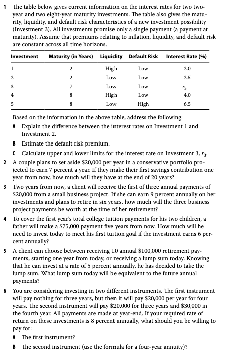
Investment 1 and 2 have the same maturity and default risks. However investment 2 has low liquidity and therefore investment 2 has a higher interest rate of 0.5% to compensate for the liquidity risk. This is the liquidity risk premium.
Problem 1B
Investment 4 and 5 have the same maturity (8 years). We know from problem 1 the liquidity risk premiums is 0.5%. The interest rate difference between Investment 4 and 5, is 2.5%. Investment 5 has low liquidity and high default risk therefore it has a higher interest rate. Since we know 0.5% is the liquidity premium, we can attribute 2.5% - 0.5% = 2% as default risk premium.
Problem 1C
Investment 2 and 3 has the same liquidity and default risk, but investment 3 has a higher maturity hence it should have atleast 2.5% as the lower bound. Investment 3 and 4 has low default risk. But investment 3 has a lower maturity and lower liquidity. We know the liquidity premium is 0.5%, but we don’t know the compensation for extra year of maturity. Therefore we could expect the interest rate for investment 3 to be between 2.5% and 4.5%.
Problem 2
library(tidyverse)

savings <- 20000
interest <- 7/100
years <- 20
timeline <- rep(20000,years)

# Create a function to calculate the future value
# of payments

get_payment_fv <- function(x,y) {

  payment <- (1 + interest) ^ (years - y) * x
  return(payment)

}

payments <- map2_dbl(.x = timeline,.y = 1:years,
                 .f = get_payment_fv)

print(timeline)
## [1] 20000 20000 20000 20000 20000 20000 20000 20000 20000 20000 20000
## [12] 20000 20000 20000 20000 20000 20000 20000 20000 20000print(payments)## [1] 72330.55 67598.65 63176.30 59043.27 55180.63 51570.68 48196.90
## [8] 45043.83 42097.04 39343.03 36769.18 34363.72 32115.63 30014.61
## [15] 28051.03 26215.92 24500.86 22898.00 21400.00 20000.00cat("The couple will have", paste0("$",round(sum(payments),2)),
"at the end of 20 years.")## The couple will have $819909.85 at the end of 20 years.Problem 3
cash_flow <- c(0, 0, 20000, 20000, 20000, 0, 0)
interest <- 9/100
years <- length(cash_flow)

payments <- map2_dbl(.x = cash_flow,
                     .y = 1:years,
                     .f = get_payment_fv)

cat("The client will have", paste0("$",round(sum(payments),2)),
    "at the end of 6 years.")
## The client will have $77894.21 at the end of 6 years.Problem 4
college_fee <- 75000
interest <- 6/100
years <- 5

pv <- (1 + interest) ^ (-years) * college_fee

cat("The father will need to invest", paste0("$",round(pv,2)),
    "today to have $75000 in 5 years at 6%")
## The father will need to invest $56044.36 today to have $75000 in 5 years at 6%Problem 5
interest <- 5/100
years <- 10

df <- tibble(year = 1:years,
       cf = rep(100000,10)) %>%
  mutate(pv = cf / (1 + interest)^ year)

print(df)
## # A tibble: 10 x 3
## year cf pv
## <int> <dbl> <dbl>
## 1 1 100000 95238.
## 2 2 100000 90703.
## 3 3 100000 86384.
## 4 4 100000 82270.
## 5 5 100000 78353.
## 6 6 100000 74622.
## 7 7 100000 71068.
## 8 8 100000 67684.
## 9 9 100000 64461.
## 10 10 100000 61391.lump_sum <- sum(df$pv)
cat("The client should expect", paste0("$",round(lump_sum, 2)), "payment today.")## The client should expect $772173.49 payment today.Problem 6A
cf1 <- c(0,0,0,rep(20000,4))

interest <- 8/100

df <- tibble(year = 1:length(cf1),
             cf = cf1) %>%
  mutate(pv = cf / (1 + interest)^ year)

print(df)
## # A tibble: 7 x 3
## year cf pv
## <int> <dbl> <dbl>
## 1 1 0 0
## 2 2 0 0
## 3 3 0 0
## 4 4 20000 14701.
## 5 5 20000 13612.
## 6 6 20000 12603.
## 7 7 20000 11670.pv <- sum(df$pv)
cat("We should be willing to pay",paste0("$",round(pv,2)),"for the first investment")## We should be willing to pay $52585.46 for the first investmentProblem 6B
cf2 <- c(rep(20000,3), 30000)
interest <- 8/100

df <- tibble(year = 1:length(cf2),
             cf = cf2) %>%
  mutate(pv = cf / (1 + interest)^ year)

cat("We should be willing to pay",paste0("$",round(pv,2)),"for the second investment")
## We should be willing to pay $52585.46 for the second investmentProblems 7 to 15 and their solution in R
Problem 7
cf <- c(rep(0,2), rep(10000,4))

interest <- 8/100

df <- tibble(year = 1:length(cf),
             cf = cf) %>%
  mutate(pv = cf / (1 + interest)^ year)

print(df)
## # A tibble: 6 x 3
## year cf pv
## <int> <dbl> <dbl>
## 1 1 0 0
## 2 2 0 0
## 3 3 10000 7938.
## 4 4 10000 7350.
## 5 5 10000 6806.
## 6 6 10000 6302.pv <- sum(df$pv)
cat("We should set aside", paste0("$",round(pv,2)), "today to pay for the college tuition")## We should set aside $28396.15 today to pay for the college tuitionProblem 8
# This is a two part problem
# First calculate the PV of
# Room and board required
# before college starts

cf1 <- rep(20000,4)
interest <- 5/100

df1 <- tibble(year = 1:length(cf1),
       cf = cf1) %>%
  mutate(pv = cf / (1 + interest)^ year)

fv <- sum(df1$pv)

cat("The client will need", fv,
    "before college starts.")
## The client will need 70919.01 before college starts.# Now we need to calculate the
# payment needed to get this
# Future value
# We will use the FV value of annuity formula
# FV = annuity((1 + r)^N - 1 / r)
# we need to make 17 payments
annuity <- fv / (((1 + interest)^17 - 1) / 0.05)
cat("The parent will need to make", paste0("$",round(annuity,2)), "to save for room and board")## The parent will need to make $2744.5 to save for room and boardProblem 9
# First we need to calculate the
# Inflation adjusted cost of college
# in the future

inflation <- 0.05
tuition_today <- 7000
college_start_years <- 18

tuition_fv_year1 <- (1 + inflation) ^ college_start_years * tuition_today

cat("Tuition will be", paste0("C$",round(tuition_fv_year1,2),
                              " for the first year, 18 years from now."))
## Tuition will be C$16846.33 for the first year, 18 years from now.# Now lets calculate the tuition payments for the next 3 years
# Year 0 is
df <- tibble(year = 1:4,
tuition = c(tuition_fv_year1, rep(0,3))) %>%
mutate(tuition = (1 + inflation)^(year - 1) * tuition_fv_year1)
print(df)## # A tibble: 4 x 2
## year tuition
## <int> <dbl>
## 1 1 16846.
## 2 2 17689.
## 3 3 18573.
## 4 4 19502.# Now we need to PV these payments at
# beginning of year 17
interest <- 6/100 # Expected returns
df <- df %>%
mutate(pv = tuition / (1 + interest) ^ year)
fv_total_tuition <- sum(df$pv)
# Now its an annuity problem as before
annuity <- fv_total_tuition / (((1 + interest)^17 - 1) / interest)
annuity## [1] 2221.579cat("The couple will need to save", paste0("$",round(annuity,2)), "each year for the expected college tuition.")## The couple will need to save $2221.58 each year for the expected college tuition.Problem 10
C. expected inflation.
Problem 11
C. Liquidity
Problem 12
(1 + 0.04/365)^365 - 1## [1] 0.04080849A. daily
Problem 13
(1+0.07 / 4) ^ (4 * 6) * 75000## [1] 113733.2A. $113733
Problem 14
100000 / (1 + 0.025 / 52) ^ 52## [1] 97531.58B. 97532
Problem 15
# Get the Effective annual rate
rate <- (1 + 0.03 / 365) ^ 365 - 1

# Get the months
# needed to quadruple the PV

log(1000000 / 250000) /  log(1 + rate) * 12
## [1] 554.5405A. 555
Problems 16 to 22 and their solution in R
Problem 16
# 3% continuously compounding
# for 4 years

continuous_compounding <- exp(0.03 * 4) * 1000000

daily_compounding <- (1 + 0.03 / 365) ^ (4 * 365) * 1000000

continuous_compounding - daily_compounding
## [1] 5.55994B. €6
Problem 17
rate <- 4/100
pmt <- 300
years <- 5

pv <- (pmt / rate * (1 - 1/(1 + rate)^years)) * (1 + rate)

pv
## [1] 1388.969B. $1389
Problem 18
quarterly_div <- 2
yearly_div <- quarterly_div * 4

# PV a year from now

fv <- yearly_div / 0.06

# Current price

pv <- fv / (1 + 0.06)
pv
## [1] 125.7862B. $126
Problem 19
rate <- 4/100
ear <- (1 + rate / 2) ^ 2

  df <- tibble(year = 1:4,
               years_remaining = 4:1,
               cf = c(4000, 8000, 7000, 10000)) %>%
  mutate(fv = cf * ((1 + 0.02) ^ ((years_remaining - 1) * 2)))

df
## # A tibble: 4 x 4
## year years_remaining cf fv
## <int> <int> <dbl> <dbl>
## 1 1 4 4000 4505.
## 2 2 3 8000 8659.
## 3 3 2 7000 7283.
## 4 4 1 10000 10000fv <- sum(df$fv)
fv## [1] 30446.91B. $30447
Problem 20
# continuously

cont <- exp(0.075 * 6) * 500000

# daily

d <- (1 + 0.07 / 365) ^ (6 * 365) * 500000

# Semiannually

s <- (1 + 0.08 / 2) ^ (6 * 2) * 500000

tibble(continuously = cont,
       daily = d,
       semiannually = s)
## # A tibble: 1 x 3
## continuously daily semiannually
## <dbl> <dbl> <dbl>
## 1 784156. 760950. 800516.C. 8.0% compounded semiannually
Problem 21
perp_payment <- 2000 / (0.06 / 12)

perp_payment
## [1] 4e+05C. greater than the lump sum
Problem 22
ordinary_annuity <- tibble(year = 1:10,
       cf = 2000) %>%
  mutate(pv = cf / (1 + 0.05) ^ year) %>%
  summarise(s = sum(pv)) %>%
  .[[1]]

annuity_due <- ordinary_annuity * 1.05
annuity_due
## [1] 16215.64B. 16216
Problems 23 to 28 and their solution in R
Problem 23
rate <- 6/100
pmt <- 50000
years <- 4
# PV of ordinary annuity
# This is also the future value

fv <- (pmt / rate * (1 - 1/(1 + rate)^years))

# Calculate the PV

pv <- fv / (1 + rate) ^ 17
pv
## [1] 64340.85B. 64341
Problem 24
rate <- 12/100

tibble(year = c(1,2,5),
       cf = c(100000, 150000, -10000)) %>%
  mutate(pv = cf / (1 + rate) ^ year) %>%
  summarise(s = sum(pv)) %>%
  .[[1]]
## [1] 203190.5B. 203191
Problem 25
rate <- 0.06/12
n <- 12 * 5

pv_factor <- (1 - (1/(1+rate) ^ n)) / rate

payment <- 200000 / pv_factor

payment
## [1] 3866.56B. 3866
Problem 26
rate <- 0.06 / 4
n = 4 * 10

25000 / (((1 + rate) ^ n - 1) / rate)
## [1] 460.6775A. 460.68
(50000 / (1 + 0.04)^20) * (1 + 0.04) ^ 5## [1] 27763.23B. $27763
Problem 28
Answer choices are
- 21670
- 22890
- 22950
p <- 0.035 * 20000
p
## [1] 700rate <- 0.02/12
n <- 4 * 12
fv_payments <- tibble(years_remaining = 3:0,
cf = p) %>%
mutate(n = years_remaining * 12) %>%
mutate(fv = (1 + rate) ^ n * cf) %>%
summarise(s = sum(fv))
20000 + fv_payments## s
## 1 22885.92B. 22890