Here are the first 6 problems and their solutions in R

library(tidyverse)

Problem 1

B. The FTSE Eurotop 100 as a representation of the European stock market

Problem 2

A. Ordinal

Problem 3

A. The 500 companies in the S&P 500 Index

Problem 4

A. median of a population.

Problem 5

df <- tibble(return_interval = c("-10 to -7", "-7 to -4", "-4 to -1", "-1 to 2", "2 to 5", "5 to 8"),
       absolute_freq = c(3,7,10,12,23,5)) %>%
  mutate(r_freq = absolute_freq / sum(.$absolute_freq)) %>%
  mutate(cum_sum = cumsum(r_freq))

df

## # A tibble: 6 x 4
##   return_interval absolute_freq r_freq cum_sum
##   <chr>                   <dbl>  <dbl>   <dbl>
## 1 -10 to -7                   3 0.05     0.05 
## 2 -7 to -4                    7 0.117    0.167
## 3 -4 to -1                   10 0.167    0.333
## 4 -1 to 2                    12 0.2      0.533
## 5 2 to 5                     23 0.383    0.917
## 6 5 to 8                      5 0.0833   1

A. The relative frequency of the interval “–1.0 to +2.0” is 20%.

Problem 6

tibble(year = 1:12,
       returns = c(2.48, -2.59, 9.47, -0.55, -1.69, -0.89, -9.19, -5.11, 1.33, 6.84, 3.04, 4.72)) %>%
  group_by(group = cut(returns, breaks = 5)) %>%
  #group_by(group = cut(returns, breaks = seq(min(returns), max(returns), length = 5))) %>%
  summarise(n = n()) %>%
  mutate(rel_freq = n / sum(.$n)) %>%
  mutate(c_freq = cumsum(rel_freq))

## # A tibble: 5 x 4
##   group             n rel_freq c_freq
##   <fct>         <int>    <dbl>  <dbl>
## 1 (-9.21,-5.46]     1   0.0833 0.0833
## 2 (-5.46,-1.73]     2   0.167  0.25  
## 3 (-1.73,2.01]      4   0.333  0.583 
## 4 (2.01,5.74]       3   0.25   0.833 
## 5 (5.74,9.49]       2   0.167  1

C. 0.5833

Problem 7

A. tabular display.

Problem 8

(2 + 7 + 15 ) / 26

## [1] 0.9230769

C. The cumulative relative frequency of Interval C is 92.3%.

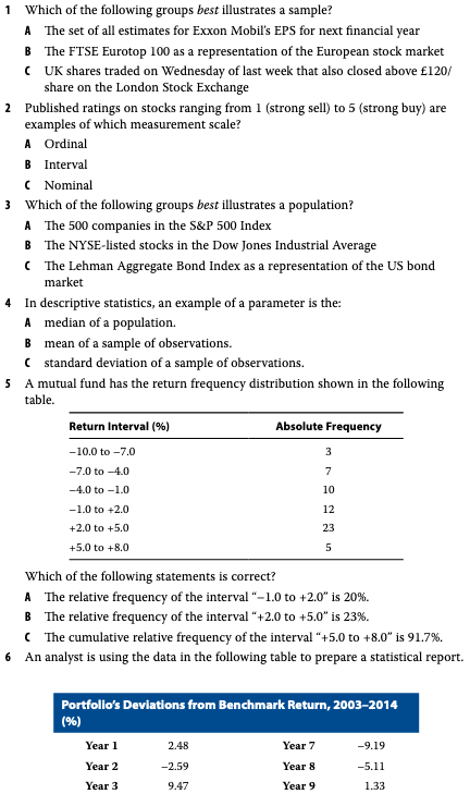
Problem 9

C. 13% to 18%

Problem 10

C. three modes

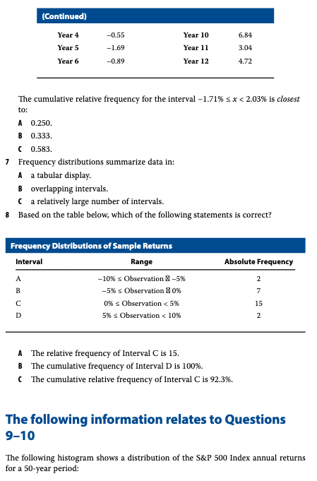
Problem 11

The following is a frequency polygon of monthly exchange rate changes in the US dollar/Japanese yen spot exchange rate for a four-year period. A positive change represents yen appreciation (the yen buys more dollars), and a negative change represents yen depreciation (the yen buys fewer dollars). (See chart above)

Based on the chart, yen appreciation: - A. occurred more than 50% of the time. - B. was less frequent than yen depreciation. - C. in the 0.0 to 2.0 interval occurred 20% of the time.

A. occurred more than 50% of the time.

Problem 12

B. absolute frequency.

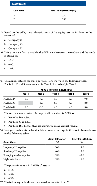
Problem 13

df <- tibble(company = c("A", "B", "C", "D", "E", "F"),
       eq_ret = c(-4.53, -1.40, -1.2, -1.2, 0.7, 8.9))
df

## # A tibble: 6 x 2
##   company eq_ret
##   <chr>    <dbl>
## 1 A        -4.53
## 2 B        -1.4 
## 3 C        -1.2 
## 4 D        -1.2 
## 5 E         0.7 
## 6 F         8.9

mean(df$eq_ret)

## [1] 0.2116667

C. Company E

Problem 14

# Median
med <- median(df$eq_ret)

# Mode is most freq value -1.2

mod <- -1.2

med - mod

## [1] 0

B. 0

Problem 15

C. Portfolio R is higher than its arithmetic mean annual return.

Problem 16

20.08.0Small- cap US equities40.012.0Emerging market equities25.0–3.0High- yield bonds15.04.0

df <- tibble(asset_class = c("Large - cap US equities", "Small - cap US equities",
                       "Emerging market equities", "High yield bonds"),
       allocation = c(20,40,25,15),
       returns = c(8,12,-3,4))

df %>%
  mutate(allocation = allocation / 100) %>%
  mutate(contribution = allocation * returns) %>%
  summarise(port_ret = sum(contribution))

## # A tibble: 1 x 1
##   port_ret
##      <dbl>
## 1     6.25

C. 6.3%

Problem 17

df <- tibble(year = 1:5,
             returns = c(19.5, -1.9, 19.7, 35, 5.7))

df %>%
  mutate(returns = returns/100) %>%
  mutate(r = 1 + returns) %>%
  mutate(cr = cumprod(r)) %>%
  select(cr) %>%
  slice(n()) %>%
  .[[1]]

## [1] 2.002349

2.002349 ** (1/5) - 1

## [1] 0.1489681

A. 14.9%

Problem 18

df <- tibble(year = 1:4,
             price = c(62,76,84,90))

df %>%
  mutate(shares = 5000 / price) %>%
  summarise(s = sum(shares)) %>%
  .[[1]]

## [1] 261.514

20000 / 261.514

## [1] 76.47774

A. $76.48

Problem 19

df <- tibble(year = 1:10,
             returns = c(15.25, 10.02, 20.65, 9.57, -40.33, 30.79, 12.34, -5.02, 16.54, 27.37))

quantile(df$returns, 0.8, type = 6)

##    80% 
## 26.026

A. 26.03%

Problem 20

df <- tibble(year = 1:10,
             returns = c(15.25, 10.02, 20.65, 9.57, -40.33, 30.79, 12.34, -5.02, 16.54, 27.37))

mean_ret <- df %>%
  filter(year >= 6) %>%
  summarise(m = mean(returns)) %>%
  .[[1]]

df %>%
  filter(year >= 6) %>%
  mutate(m = abs(returns - mean_ret)) %>%
  summarise(mm = mean(m))

## # A tibble: 1 x 1
##      mm
##   <dbl>
## 1  10.2

A. 10.20 %

Problem 21

df <- tibble(returns = c(-38.49, -0.73, 0.00, 9.54, 11.39, 12.78, 13.41, 19.42, 23.45, 29.60))
df

## # A tibble: 10 x 1
##    returns
##      <dbl>
##  1  -38.5 
##  2   -0.73
##  3    0   
##  4    9.54
##  5   11.4 
##  6   12.8 
##  7   13.4 
##  8   19.4 
##  9   23.4 
## 10   29.6

quantile(df$returns, type = 6)

##       0%      25%      50%      75%     100% 
## -38.4900  -0.1825  12.0850  20.4275  29.6000

B. 20.44%

Problem 22

sp_range <- abs(min(df$returns) - max(df$returns))
sp_mad <- mad(df$returns, center = mean(df$returns))

sp_range

## [1] 68.09

sp_mad

## [1] 12.45681

C. MAD and range

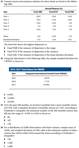
Problem 23

abc <- c(-20,23,-14,5,-14)
xyz <- c(-33,-12,-12,-8,11)
pqr <- c(-14,-18,6,-2,3)

get_stats <- function(x,y) {
  
  r <- abs(min(x) - max(x))
  v <- var(x)
  m <- mad(x, center = mean(x))
  
  cat(r,v,m,"for",y)
}

get_stats(abc,'abc')

## 43 316.5 14.826 for abc

get_stats(xyz,'xyz')

## 44 244.7 4.15128 for xyz

get_stats(pqr,'pqr')

## 24 111 13.3434 for pqr

C. Fund ABC if the measure of dispersion is the mean absolute deviation.

Problem 24

ret <- c(-0.67, 1.71, 42.96)

sd(ret)

## [1] 24.53163

C. 24.54

Problem 25

mean_ret <-  0.79
sd_ret <- 1.16
upper_limit <- 2.53 - mean_ret

lower_limit <- -0.95 - mean_ret

k <- upper_limit / sd_ret

(1 - 1/k^2) * 240

## [1] 133.3333

C. 133

Problem 26

k <- 8/4

(1 - 1/k^2) * 2000

## [1] 1500

B. 1500

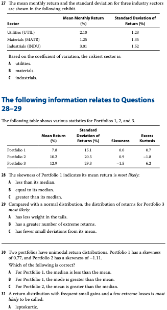
Problem 27

df <- tibble(sector = c("utilities", "materials", "industrials"),
             mean_ret = c(2.1, 1.25, 3.01),
             sd_ret = c(1.23, 1.35, 1.52))

df %>%
  mutate(v = sd_ret / mean_ret)

## # A tibble: 3 x 4
##   sector      mean_ret sd_ret     v
##   <chr>          <dbl>  <dbl> <dbl>
## 1 utilities       2.1    1.23 0.586
## 2 materials       1.25   1.35 1.08 
## 3 industrials     3.01   1.52 0.505

B. matrials

Problem 28

B. equal to its median.

Problem 29

B. has a greater number of extreme returns

Problem 30

A. For Portfolio 1, the median is less than the mean.

Problem 31

C. negatively skewed.

Problem 32

B. mode < median < mean

Problem 33

B. platykurtic

Problem 34

B. The geometric mean measures an investment’s compound rate of growth over multiple periods.

Problem 35

B. Geometric