Downloading the stock price for Netflix

Netflix has seen phenomenal growth since 2009. It was responsible for producing a new category of business - subscription based online streaming. It has changed the industry landscape and pushed Blockbuster our of business. Old media companies like CBS, Fox, Viacom, Disney etc are under threat from the new way of consuming media. Netflix started as a content delivery platform, but today its responsible for content creation as well. Its original programs have won several Emmy awards. Today Netflix seems like an unstoppable force in the media landscape.

To see just how well Netflix’s stock has performed, we will start by downloading the historical price for Netflix and then perform the return calculations.

netflix = web.get_data_yahoo("NFLX",
                            start = "2009-01-01",
                            end = "2018-03-01")

print(netflix.head())

##                 High       Low    ...          Volume  Adj Close
## Date                              ...                           
## 2009-01-02  4.357143  4.200000    ...       6605200.0   4.267143
## 2009-01-05  4.562857  4.302857    ...      13044500.0   4.562857
## 2009-01-06  4.750000  4.590000    ...      12065900.0   4.705714
## 2009-01-07  4.734286  4.571429    ...      10133900.0   4.672857
## 2009-01-08  4.797143  4.485714    ...       8175300.0   4.735714
## 
## [5 rows x 6 columns]

Next we will chart the Netflix’s adjusted closing price.

netflix['Adj Close'].plot()
plt.xlabel("Date")
plt.ylabel("Adjusted")
plt.title("Netflix Price data")
plt.show()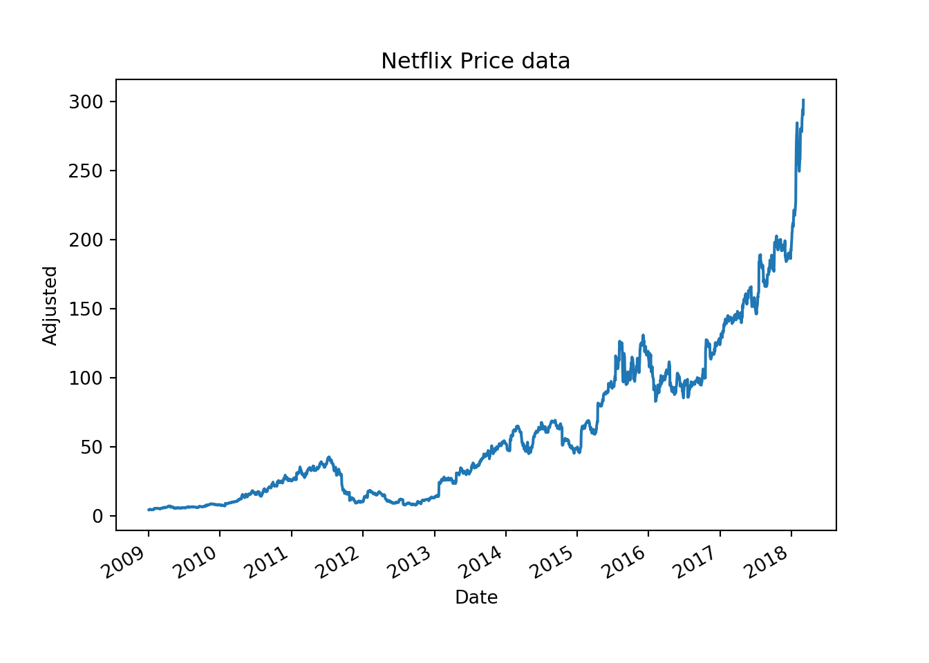

Calculating the daily and monthly returns for individual stock

Once we downloaded the stock prices from yahoo finance, the next thing to do is to calculate the returns. We will again use pandas package to do the calculations. We have already downloaded the price data for Netflix above, if you haven’t done that then see the above section. We will calculate the monthly and daily price returns.

netflix_daily_returns = netflix['Adj Close'].pct_change()
netflix_monthly_returns = netflix['Adj Close'].resample('M').ffill().pct_change()

Looking at the head of the daily returns.

print(netflix_daily_returns.head())

## Date
## 2009-01-02         NaN
## 2009-01-05    0.069300
## 2009-01-06    0.031309
## 2009-01-07   -0.006982
## 2009-01-08    0.013452
## Name: Adj Close, dtype: float64

Looking at the head of the monthly returns.

print(netflix_monthly_returns.head())

## Date
## 2009-01-31         NaN
## 2009-02-28    0.002767
## 2009-03-31    0.184327
## 2009-04-30    0.055685
## 2009-05-31   -0.129993
## Freq: M, Name: Adj Close, dtype: float64

Charting the daily and monthly for Netflix

fig = plt.figure()
ax1 = fig.add_axes([0.1,0.1,0.8,0.8])
ax1.plot(netflix_daily_returns)
ax1.set_xlabel("Date")
ax1.set_ylabel("Percent")
ax1.set_title("Netflix daily returns data")
plt.show()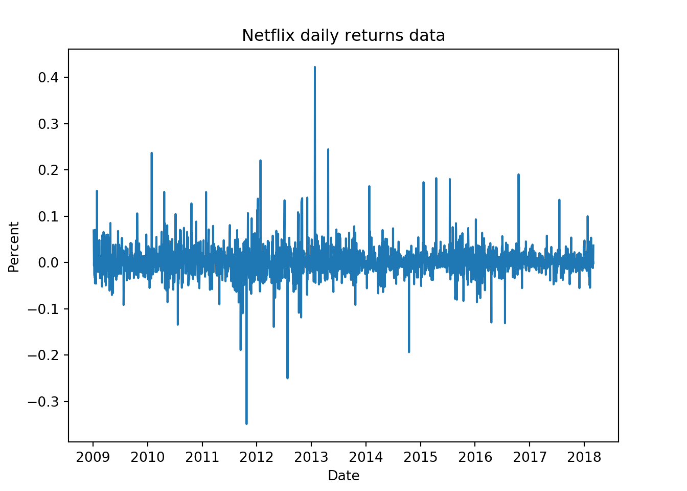

fig = plt.figure()
ax1 = fig.add_axes([0.1,0.1,0.8,0.8])
ax1.plot(netflix_monthly_returns)
ax1.set_xlabel("Date")
ax1.set_ylabel("Percent")
ax1.set_title("Netflix monthly returns data")
plt.show()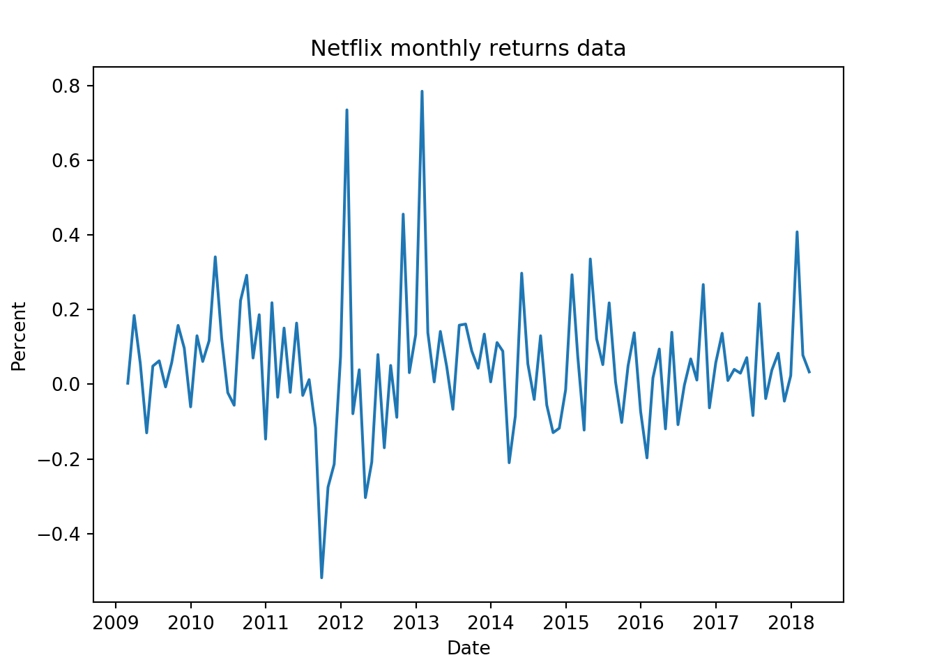

After looking at the daily returns chart for Netflix we can conclude that the returns are quite volatile and the stock can move +/- 5% on any given day. To get a sense of how extreme the returns can be we can plot a histogram.

fig = plt.figure()
ax1 = fig.add_axes([0.1,0.1,0.8,0.8])
netflix_daily_returns.plot.hist(bins = 60)
ax1.set_xlabel("Daily returns %")
ax1.set_ylabel("Percent")
ax1.set_title("Netflix daily returns data")
ax1.text(-0.35,200,"Extreme Low\nreturns")
ax1.text(0.25,200,"Extreme High\nreturns")
plt.show()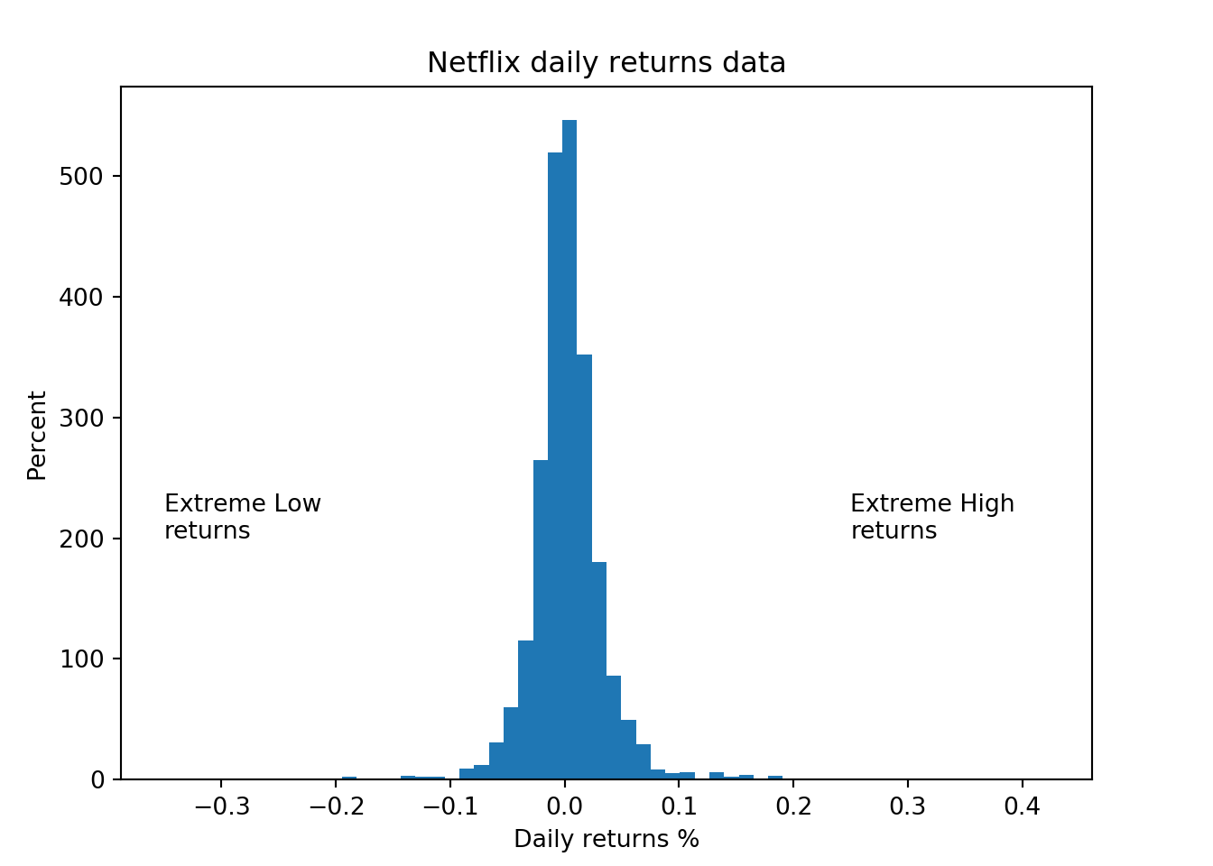

Calculating the cumulative returns for the Netflix stock

Plotting the daily and monthly returns are useful for understanding the daily and monthly volatility of the investment. To calculate the growth of our investment or in other word, calculating the total returns from our investment, we need to calculate the cumulative returns from that investment. To calculate the cumulative returns we will use the cumprod() function.

netflix_cum_returns = (netflix_daily_returns + 1).cumprod()

Next we can chart the cumulative returns of Netflix.

fig = plt.figure()
ax1 = fig.add_axes([0.1,0.1,0.8,0.8])
netflix_cum_returns.plot()
ax1.set_xlabel("Date")
ax1.set_ylabel("Growth of $1 investment")
ax1.set_title("Netflix daily cumulative returns data")
plt.show()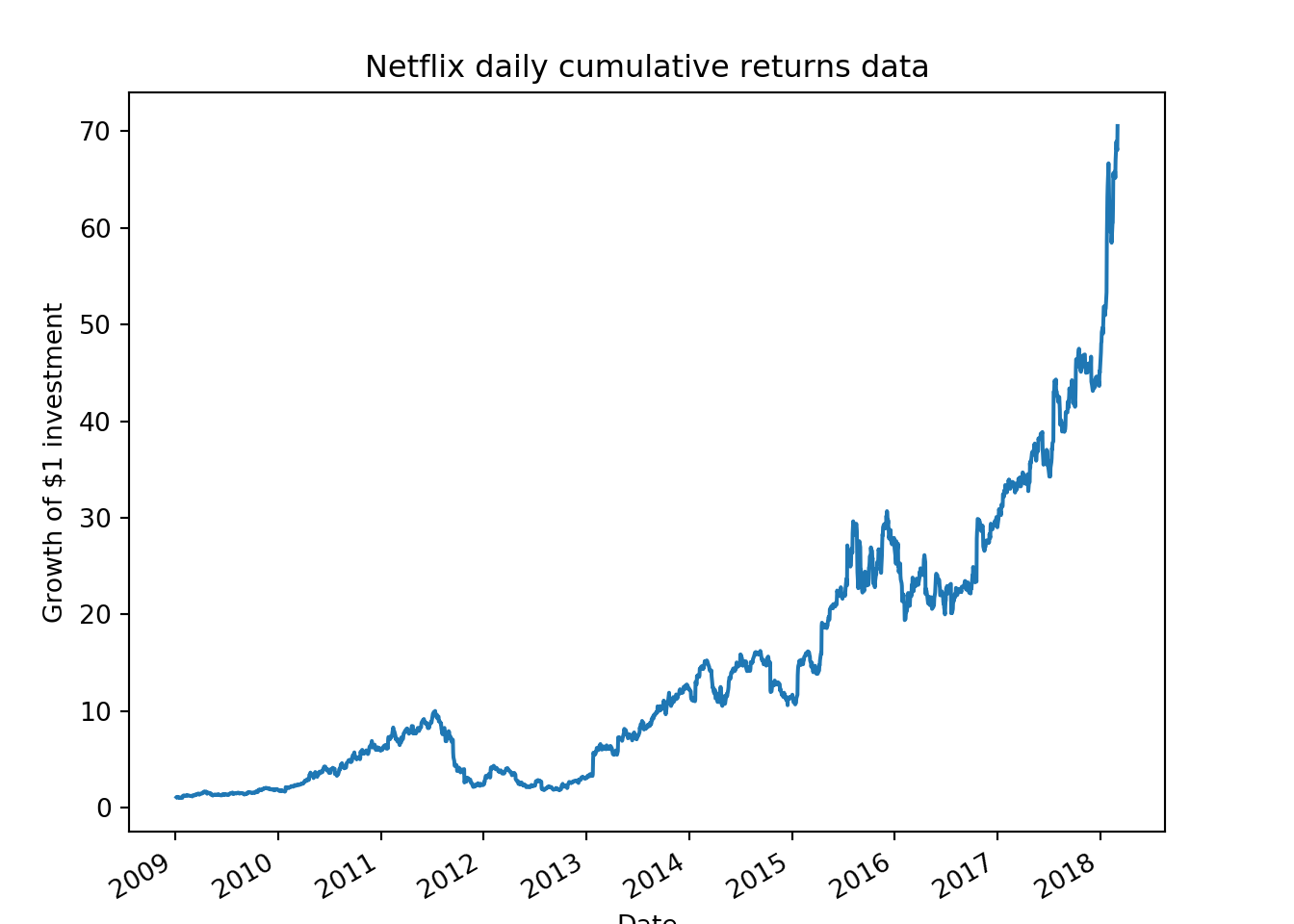

This chart shows the cumulative returns since 2009 for Netflix. With the power of hindsight, one could have made $70 on a $1 investment since 2009. That is quite a remarkable performance. But as we know its easier said then done. During the 10 year or so period there were times when the investment lost 50% of its value during the Qwickster fiasco. Very few investors can hold onto investments through such periods.

fig = plt.figure()
ax1 = fig.add_axes([0.1,0.1,0.8,0.8])
netflix_cum_returns = (netflix_monthly_returns + 1).cumprod()
ax1.plot(netflix_cum_returns)
ax1.set_xlabel("Date")
ax1.set_ylabel("Growth of $1 investment")
ax1.set_title("Netflix Monthly cumulative returns data")
plt.show()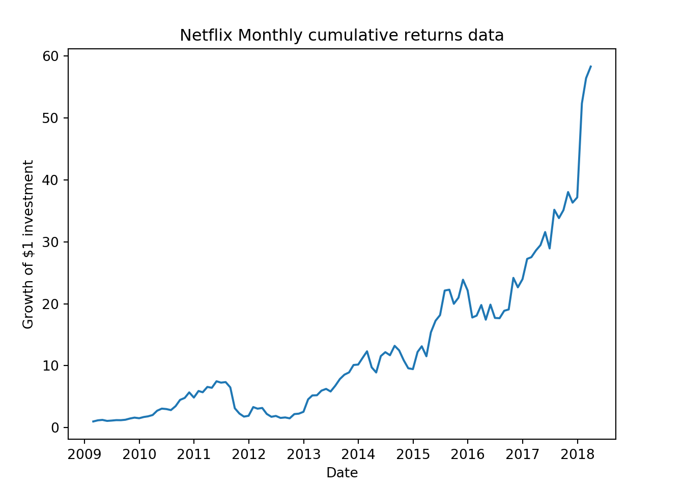

We can visualize that the monthly returns chart is much more smoother than the daily chart.

Downloading stock market data for multiple stocks.

We can download the financial data for multiple stocks. We first assign the stock symbols to a variable named “tickers”", and use that to download the stock prices.

tickers = ["FB", "AMZN", "AAPL", "NFLX", "GOOG"]
multpl_stocks = web.get_data_yahoo(tickers,
start = "2013-01-01",
end = "2018-03-01")

Charting the stock prices for multiple stocks

Next we will chart the stock prices for multiple stocks

fig = plt.figure()
ax1 = fig.add_subplot(321)
ax2 = fig.add_subplot(322)
ax3 = fig.add_subplot(323)
ax4 = fig.add_subplot(324)
ax5 = fig.add_subplot(325)
ax1.plot(multpl_stocks['Adj Close']['AMZN'])
ax1.set_title("Amazon")
ax2.plot(multpl_stocks['Adj Close']['AAPL'])
ax2.set_title("Apple")
ax3.plot(multpl_stocks['Adj Close']['FB'])
ax3.set_title("Facebook")
ax4.plot(multpl_stocks['Adj Close']['NFLX'])
ax4.set_title("Netflix")
ax5.plot(multpl_stocks['Adj Close']['GOOG'])
ax5.set_title("Google")
plt.tight_layout()
plt.show()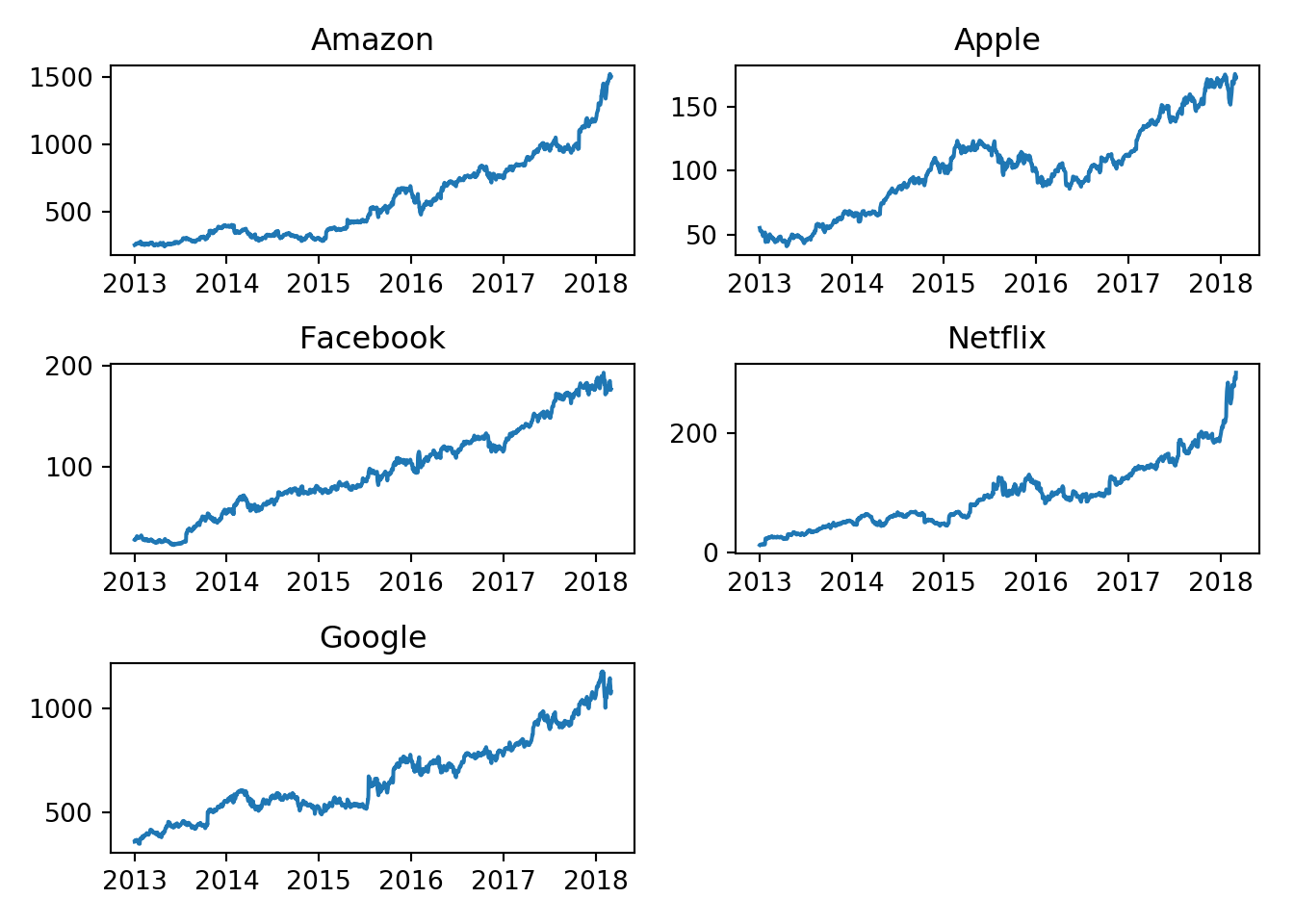

Calculating the returns for multiple stocks

Calculating the the returns for multiple stocks is just as easy as the single stock.

multpl_stock_daily_returns = multpl_stocks['Adj Close'].pct_change()
multpl_stock_monthly_returns = multpl_stocks['Adj Close'].resample('M').ffill().pct_change()

fig = plt.figure()
(multpl_stock_monthly_returns + 1).cumprod().plot()
plt.show()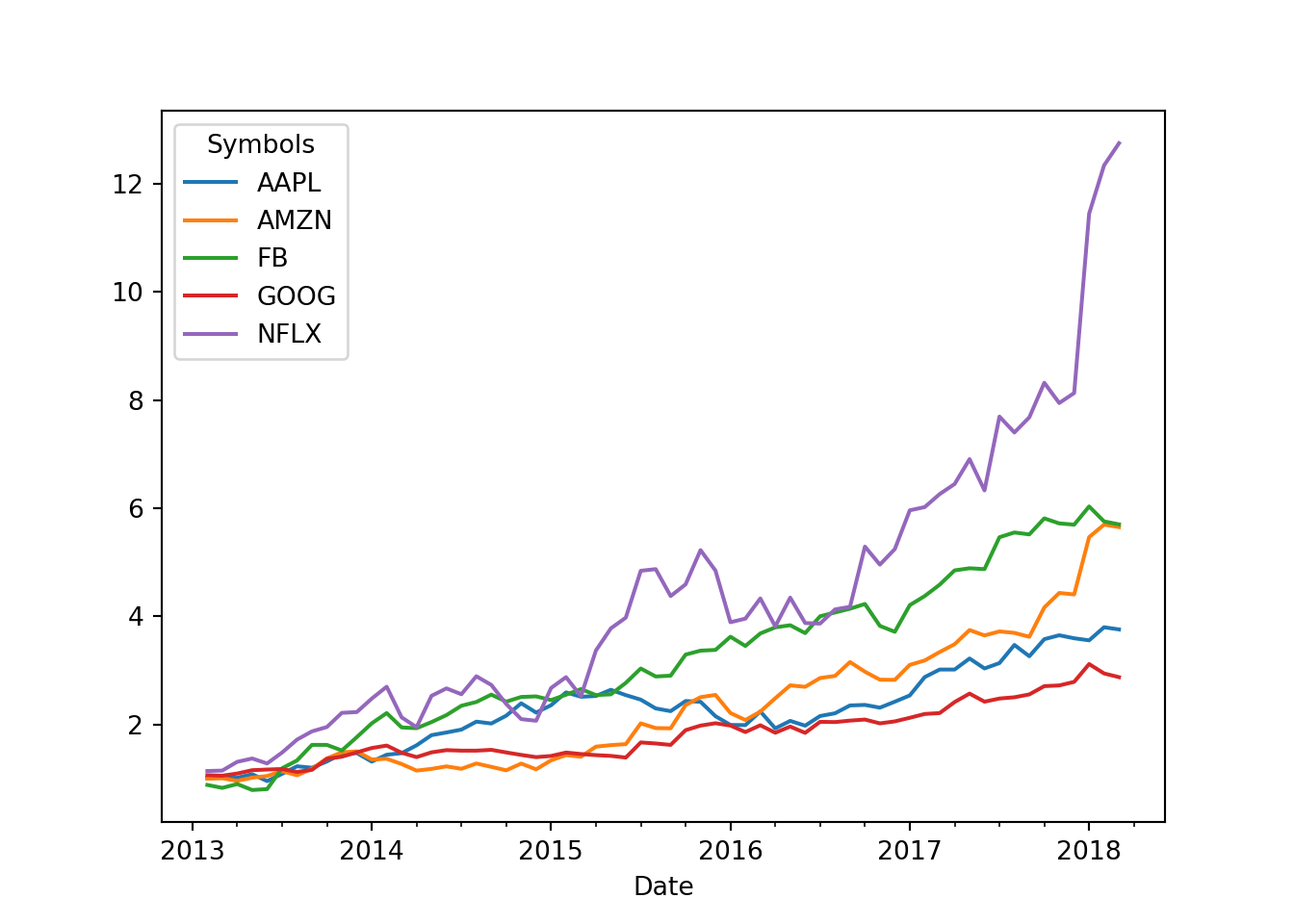

Not surprisingly, Netflix had the best returns since 2013. Amazon and Facebook come in distant second and third. The most surprising result is Google. It has severely under performed the other stocks in the FAANG group. Maybe the market participants are worried about its spending on the moon shot projects (Google glass, X Labs, Waymo etc). Whether these projects can produce results is yet to be seen.

A contrarian could argue that given the investments in the future projects, Google is currently undervalued an could be the better investment among the FAANG stocks.

Calculating the Mean, standard deviation and other stats

We already have the daily and monthly returns data for Netflix. Now we we will calculate the daily and monthly mean and standard deviations of the returns. We will use mean() and std() functions for our purpose.

print(multpl_stock_monthly_returns.mean())

## Symbols
## AAPL    0.023860
## AMZN    0.031329
## FB      0.031989
## GOOG    0.018693
## NFLX    0.049129
## dtype: float64

print(multpl_stock_monthly_returns.std())

## Symbols
## AAPL    0.068283
## AMZN    0.080158
## FB      0.089625
## GOOG    0.056989
## NFLX    0.125132
## dtype: float64