Calculating portfolio returns using the formula

A portfolio return is the weighted average of individual assets in the portfolio.

Here is what we need

• Asset symbols that make up our portfolio
• Price data for the assets
• weights of assets
• Calculating the weighted average of our assets returns
• Adding them to get the portfolio returns

Lets first load the packages

library(tidyquant)

We will invest in the following assets

• Aggregate Bonds ETF (BND) 10%
• Small Cap ETF (VB) 20%
• Developed markets ETF (VEA) 25%
• S&P 500 ETF (VOO) 25%
• Emerging Markets ETF (VWO) 20%

So lets assign our ticker symbols and weights.

# Asset tickers
tickers = c('BND', 'VB', 'VEA', 'VOO', 'VWO')

# Asset weights

wts = c(0.1,0.2,0.25,0.25,0.2)

Next we will download the price data

price_data <- tq_get(tickers,
                     from = '2013-01-01',
                     to = '2018-03-01',
                     get = 'stock.prices')

Then we will calculate the returns for our assets. We will calculate the daily returns.

ret_data <- price_data %>%
  group_by(symbol) %>%
  tq_transmute(select = adjusted,
               mutate_fun = periodReturn,
               period = "daily",
               col_rename = "ret")

Lets take a look at the first and second row of each asset in our returns data.

ret_data %>%
  group_by(symbol) %>%
  slice(c(1,2))

## # A tibble: 10 x 3
## # Groups:   symbol [5]
##    symbol date             ret
##    <chr>  <date>         <dbl>
##  1 BND    2013-01-02  0       
##  2 BND    2013-01-03 -0.00298 
##  3 VB     2013-01-02  0       
##  4 VB     2013-01-03 -0.000601
##  5 VEA    2013-01-02  0       
##  6 VEA    2013-01-03 -0.0101  
##  7 VOO    2013-01-02  0       
##  8 VOO    2013-01-03 -0.000898
##  9 VWO    2013-01-02  0       
## 10 VWO    2013-01-03 -0.00594

Next we will have to add the weight column to our returns data. For that we will create a new weights table and then join that to our returns data table.

wts_tbl <- tibble(symbol = tickers,
                  wts = wts)
head(wts_tbl)

## # A tibble: 5 x 2
##   symbol   wts
##   <chr>  <dbl>
## 1 BND     0.1 
## 2 VB      0.2 
## 3 VEA     0.25
## 4 VOO     0.25
## 5 VWO     0.2

Now lets join this to our returns data table.

ret_data <- left_join(ret_data,wts_tbl, by = 'symbol')

Again lets look at the first and second row of our table.

ret_data %>%
  group_by(symbol) %>%
  slice(c(1,2))

## # A tibble: 10 x 4
## # Groups:   symbol [5]
##    symbol date             ret   wts
##    <chr>  <date>         <dbl> <dbl>
##  1 BND    2013-01-02  0         0.1 
##  2 BND    2013-01-03 -0.00298   0.1 
##  3 VB     2013-01-02  0         0.2 
##  4 VB     2013-01-03 -0.000601  0.2 
##  5 VEA    2013-01-02  0         0.25
##  6 VEA    2013-01-03 -0.0101    0.25
##  7 VOO    2013-01-02  0         0.25
##  8 VOO    2013-01-03 -0.000898  0.25
##  9 VWO    2013-01-02  0         0.2 
## 10 VWO    2013-01-03 -0.00594   0.2

We can see that the weights have been correctly added to the corresponding assets. Now lets multiply the two columns to get our weighted average.

ret_data <- ret_data %>%
  mutate(wt_return = wts * ret)

Lets take a quick look at the result of our operation.

ret_data %>%
  group_by(symbol) %>%
  slice(c(1,2))

## # A tibble: 10 x 5
## # Groups:   symbol [5]
##    symbol date             ret   wts wt_return
##    <chr>  <date>         <dbl> <dbl>     <dbl>
##  1 BND    2013-01-02  0         0.1   0       
##  2 BND    2013-01-03 -0.00298   0.1  -0.000298
##  3 VB     2013-01-02  0         0.2   0       
##  4 VB     2013-01-03 -0.000601  0.2  -0.000120
##  5 VEA    2013-01-02  0         0.25  0       
##  6 VEA    2013-01-03 -0.0101    0.25 -0.00251 
##  7 VOO    2013-01-02  0         0.25  0       
##  8 VOO    2013-01-03 -0.000898  0.25 -0.000225
##  9 VWO    2013-01-02  0         0.2   0       
## 10 VWO    2013-01-03 -0.00594   0.2  -0.00119

We now have a weighted returns column. Now the portfolio return for each day is simply the sum of the weighted returns each day. Lets add that and get our portfolio returns.

port_ret <- ret_data %>%
  group_by(date) %>%
  summarise(port_ret = sum(wt_return))

head(port_ret)

## # A tibble: 6 x 2
##   date       port_ret
##   <date>        <dbl>
## 1 2013-01-02  0      
## 2 2013-01-03 -0.00434
## 3 2013-01-04  0.00448
## 4 2013-01-07 -0.00432
## 5 2013-01-08 -0.00402
## 6 2013-01-09  0.00395

Now we have just calculated the portfolio returns using a manual process. Lets visualize the returns.

port_ret %>%
  ggplot(aes(x = port_ret)) + 
  geom_histogram(bins = 60) +
  theme_light() +
  labs(x = "Portfolio Returns",
       y = "Frequency",
       title = "Daily Portfolio returns histogram")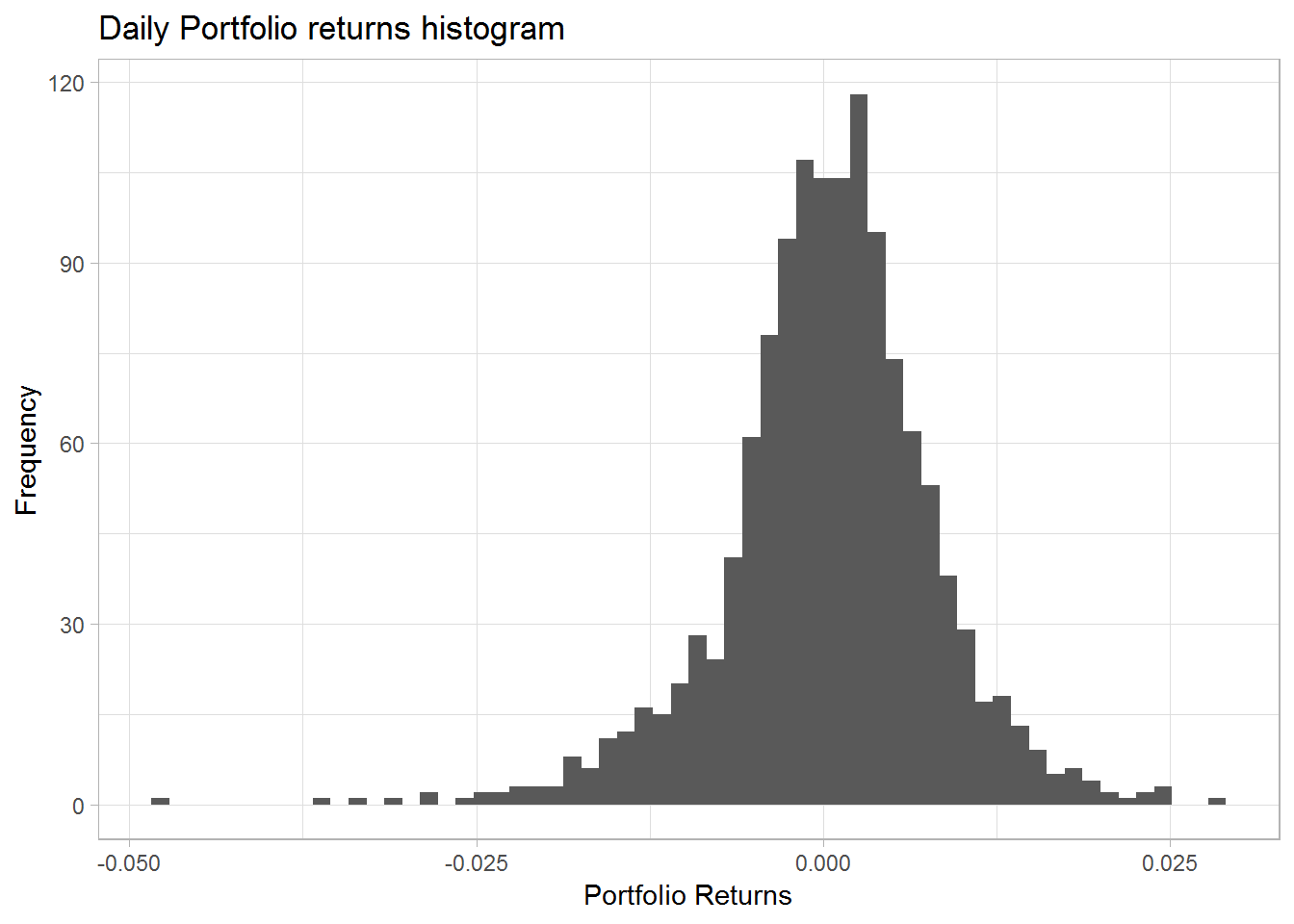

We will analyze the portfolio returns little more in the post but right now we will show you a simpler way to calculate the portfolio returns using the tidyquant package.

tidyquant helps us eliminate the extra steps we took to add the weights columns and do the multiplication and the additions.

So lets see how we will do this in tidyquant

port_ret_tidy <- price_data %>%
  group_by(symbol) %>%
  tq_transmute(select = adjusted,
               mutate_fun = periodReturn,
               period = "daily",
               col_rename = "ret") %>%
  #Using tq_portfolio from tidyquant
  tq_portfolio(assets_col = symbol,
               returns_col = ret,
               weights = wts,
               geometric = FALSE,
               col_rename = 'port_ret')

As you will notice the first part is similar to what we did before, but then we simply used tq_portfolio to calculate our portfolio returns. Here we have to specify the asset column, the returns column and the weights to calculate the portfolio returns. We will demonstrate that the returns are the same by taking the difference between two methods. First we show the histogram of the returns and the we plot the time series.

port_ret_tidy %>%
  ggplot(aes(x = port_ret)) + 
  geom_histogram(bins = 60) +
  theme_light() +
  labs(x = "Portfolio Returns",
       y = "Frequency",
       title = "Daily Portfolio returns histogram\nCalculated using tidyquant")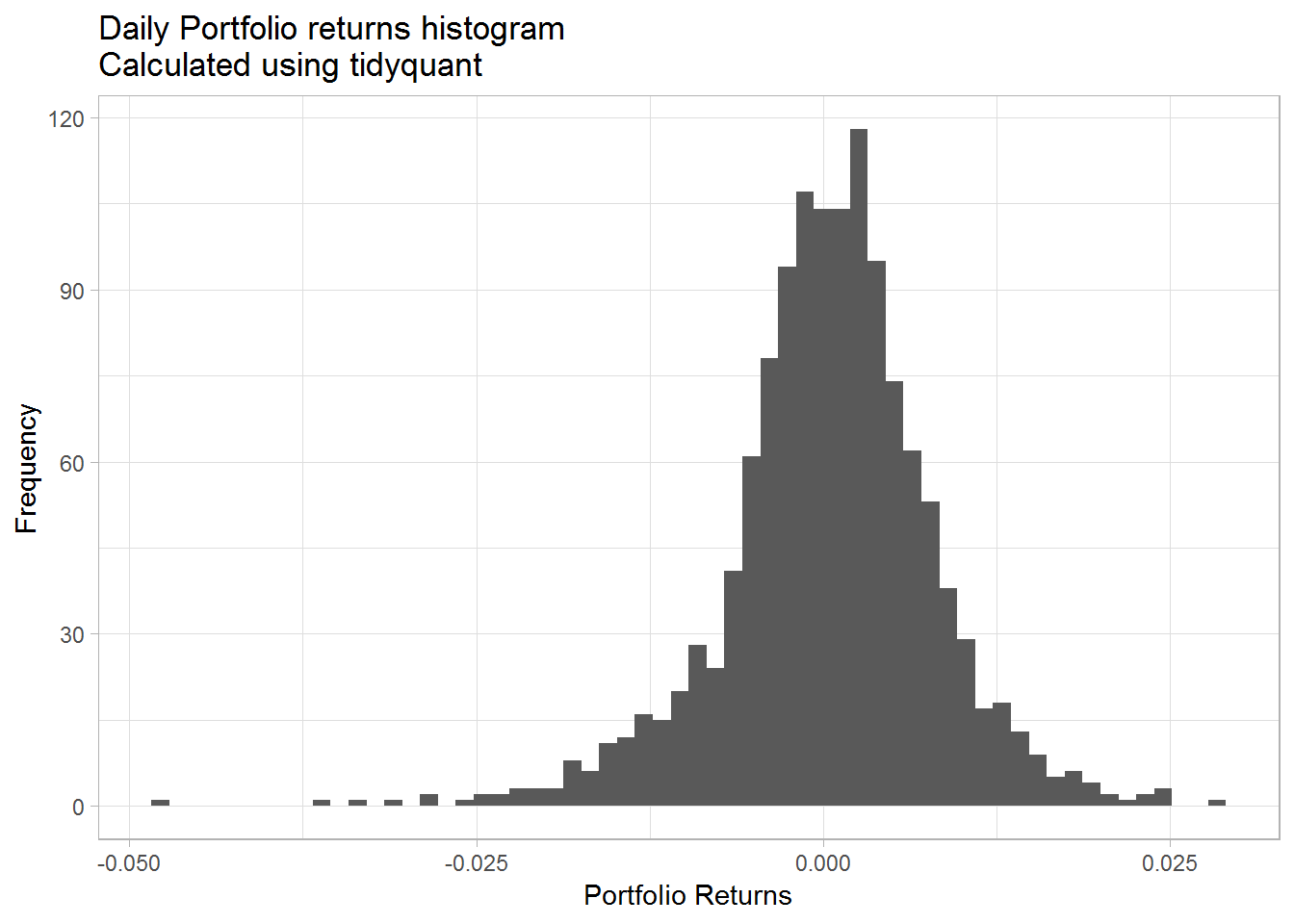

diff = port_ret$port_ret - port_ret_tidy$port_ret

unique(diff)

## [1] 0

We can see the difference between the two methods is 0.

Portfolio mean returns and standard deviation

Now that we are confident about our work, lets calculate the mean returns and the standard deviation of the portfolio.

mean(port_ret_tidy$port_ret, na.rm = TRUE)

## [1] 0.0003789623

sd(port_ret_tidy$port_ret, na.rm = TRUE)

## [1] 0.007586083

We will conclude this post here and in the next post we will analyze our portfolio further.