In this post we will calculate the portfolio beta

As usual we will start with loading our libraries.

library(tidyquant)
library(timetk)

We will use the same assets from the last post to build our portfolio.

# Create the tickers and weights vector

tickers = c('BND', 'VB', 'VEA', 'VOO', 'VWO')

wts = c(0.1,0.2,0.25,0.25,0.2)

Next lets download the price data from yahoo finance.

price_data <- tq_get(tickers,
                     from = '2013-01-01',
                     to = '2018-03-01',
                     get = 'stock.prices')

Then we will calculate the daily returns for our assets.

ret_data <- price_data %>%
  group_by(symbol) %>%
  tq_transmute(select = adjusted,
               mutate_fun = periodReturn,
               period = "daily",
               col_rename = "ret")

We will use the tq_portfolio package to quickly calculate the portfolio returns.

port_ret <- ret_data %>%
  tq_portfolio(assets_col = symbol,
               returns_col = ret,
               weights = wts,
               col_rename = 'port_ret',
               geometric = FALSE)

In order to calculate the portfolio beta, we need to regress the portfolio returns against the benchmark returns. To do that we will use S&P 500 etf as our benchmark and calculate its returns.

# Downloading benchmark price

bench_price <- tq_get('SPY',
                      from = '2013-01-01',
                      to = '2018-03-01',
                      get = 'stock.prices')

# Calculating benchmark returns

bench_ret <- bench_price %>%
  tq_transmute(select = adjusted,
               mutate_fun = periodReturn,
               period = "daily",
               col_rename = "bench_ret")

Next we need to create a table with portfolio returns and the benchmark returns. We will use the left_join to create this table.

comb_ret <- left_join(port_ret,bench_ret, by = 'date')

We can visualize the scatter plot of our portfolio returns versus benchmark returns.

comb_ret %>%
  ggplot(aes(x = bench_ret,
             y = port_ret)) +
  geom_point(alpha = 0.3) +
  geom_smooth(method = 'lm',
              se = FALSE) +
  theme_classic() +
  labs(x = 'Benchmark Returns',
       y = "Portfolio Returns",
       title = "Portfolio returns vs Benchmark returns") +
  scale_x_continuous(breaks = seq(-0.1,0.1,0.01),
                     labels = scales::percent) +
  scale_y_continuous(breaks = seq(-0.1,0.1,0.01),
                     labels = scales::percent)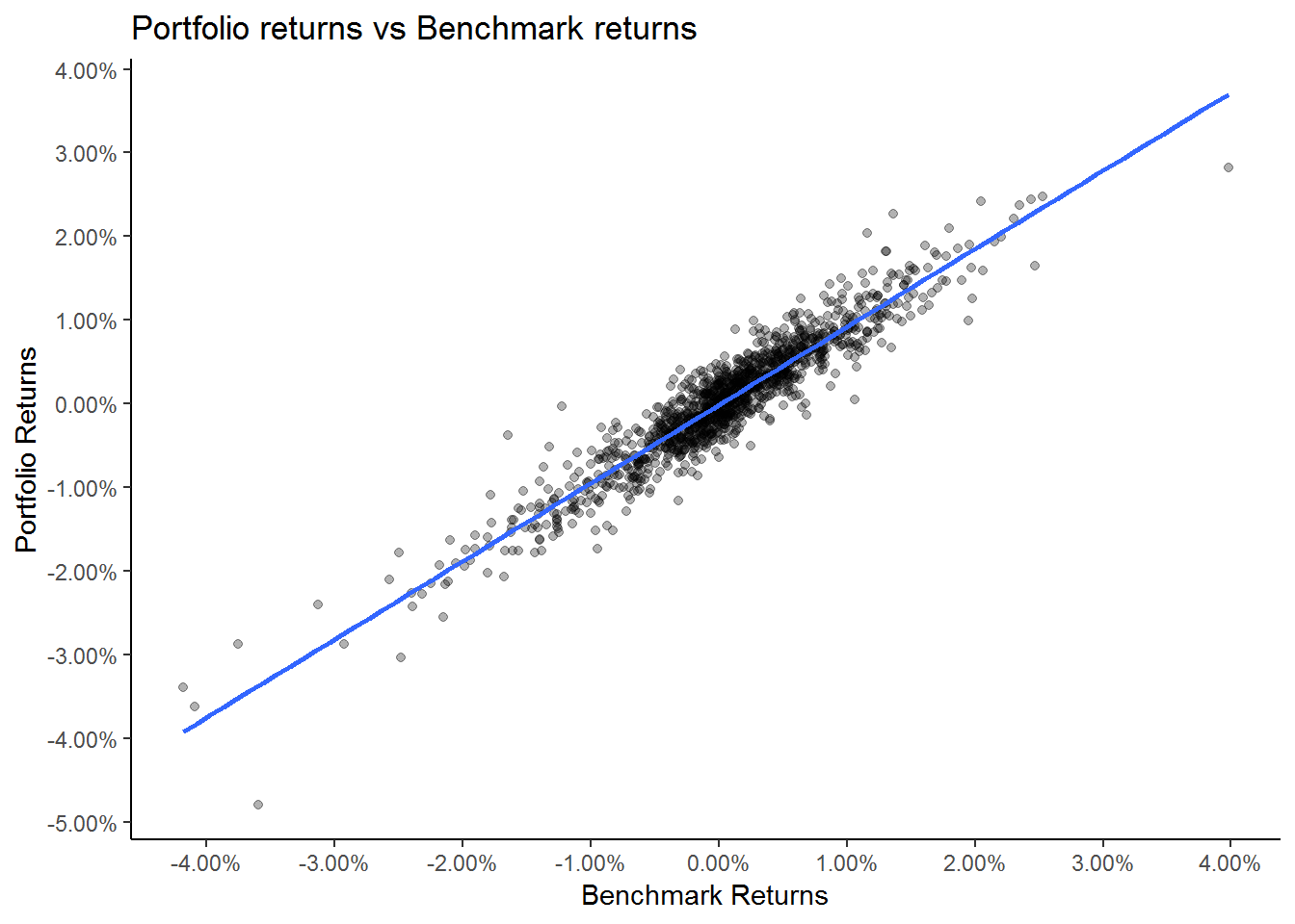

We can see that our portfolio returns are highly correlated to the benchmark returns. We can use the regression model to calculate the portfolio beta and the portfolio alpha. We will us the linear regression model to calculate the alpha and the beta.

model <- lm(comb_ret$port_ret ~ comb_ret$bench_ret)

model_alpha <- model$coefficients[1]

model_beta <- model$coefficients[2]

cat("The portfolio alpha is", model_alpha, "and the portfolio beta is", model_beta)

## The portfolio alpha is -0.0001668939 and the portfolio beta is 0.9341724

We can see that this portfolio had a negative alpha. The portfolio beta was 0.93. This suggests that for every +1% move in the S&P 500 our portfolio will go up 0.93% in value.