Web scraping is an essential skill that is required for data exploration and analysis. In this post we will learn how to get the data from a website in R for further research.

Suppose we want to get all the S&P 500 constituents for our portfolio research. This information is easily available on Wikipedia.com. Using the the below code we can download the tickers and other relevant data from wikipedia.

First lets load the libraries

library(tidyverse)
library(timetk)
library(rvest) # required for web scraping

Next we will write our code to get the Wikipedia table.

# Go to the website and read the html page
url <- "https://en.wikipedia.org/wiki/List_of_S%26P_500_companies"
url <- read_html(url)

# Get the correct data table, 
# We want the table which has
# the constituents
raw_data <- url %>%
  html_nodes("#constituents td") %>%
  html_text()

# After getting the data
# Convert the vector into a matrix

raw_data <- matrix(raw_data, ncol = 9, byrow = TRUE)

# Convert the matrix into a tibble
raw_data <- data.frame(raw_data, stringsAsFactors = FALSE) %>%
  tk_tbl()
  
# Read the head of the data table

head(raw_data)

## # A tibble: 6 x 9
##   X1     X2       X3     X4        X5         X6        X7    X8    X9    
##   <chr>  <chr>    <chr>  <chr>     <chr>      <chr>     <chr> <chr> <chr> 
## 1 "MMM\~ 3M Comp~ repor~ Industri~ Industria~ St. Paul~ ""    0000~ "1902~
## 2 "ABT\~ Abbott ~ repor~ Health C~ Health Ca~ North Ch~ 1964~ 0000~ "1888~
## 3 "ABBV~ AbbVie ~ repor~ Health C~ Pharmaceu~ North Ch~ 2012~ 0001~ "2013~
## 4 "ABMD~ ABIOMED~ repor~ Health C~ Health Ca~ Danvers,~ 2018~ 0000~ "1981~
## 5 "ACN\~ Accentu~ repor~ Informat~ IT Consul~ Dublin, ~ 2011~ 0001~ "1989~
## 6 "ATVI~ Activis~ repor~ Communic~ Interacti~ Santa Mo~ 2015~ 0000~ "2008~

We have successfully downloaded the data and now we need to do some cleaning.

# Change the column names

colnames(raw_data) <- c('symbol', 'name', 'sec_report', 'GICS_Sector', 'GICS_SubIndustry', 'headquarters', 'date_first_added', 'CIK', 'year_founded')

head(raw_data)

## # A tibble: 6 x 9
##   symbol name  sec_report GICS_Sector GICS_SubIndustry headquarters
##   <chr>  <chr> <chr>      <chr>       <chr>            <chr>       
## 1 "MMM\~ 3M C~ reports    Industrials Industrial Cong~ St. Paul, M~
## 2 "ABT\~ Abbo~ reports    Health Care Health Care Equ~ North Chica~
## 3 "ABBV~ AbbV~ reports    Health Care Pharmaceuticals  North Chica~
## 4 "ABMD~ ABIO~ reports    Health Care Health Care Equ~ Danvers, Ma~
## 5 "ACN\~ Acce~ reports    Informatio~ IT Consulting &~ Dublin, Ire~
## 6 "ATVI~ Acti~ reports    Communicat~ Interactive Hom~ Santa Monic~
## # ... with 3 more variables: date_first_added <chr>, CIK <chr>,
## #   year_founded <chr>

Next we will remove the \n new line from the ticker and the year founded columns and delete the sec_report column.

raw_data <- raw_data %>%
  select(-sec_report) %>%
  mutate(symbol = str_remove(.$symbol, '\n')) %>%
  mutate(year_founded = str_remove(.$year_founded, '\n'))

Finally lets convert the date first added and year founded to correct date format.

# Load the lubridate package
# For date formatting

library(lubridate)

raw_data <- raw_data %>%
  mutate(date_first_added = ymd(date_first_added))

# Since we are given just the year for
# the founding, we will assume 
# Founding day/month as 1st Jan

raw_data <- raw_data %>%
  mutate(year_founded = str_sub(.$year_founded,start = 1,end = 4)) %>%
  mutate(year_founded = make_date(year = year_founded,month = 1,day = 1))

# Saving it into a new table

sp_constituents <- raw_data

sp_constituents

## # A tibble: 505 x 8
##    symbol name  GICS_Sector GICS_SubIndustry headquarters date_first_added
##    <chr>  <chr> <chr>       <chr>            <chr>        <date>          
##  1 MMM    3M C~ Industrials Industrial Cong~ St. Paul, M~ NA              
##  2 ABT    Abbo~ Health Care Health Care Equ~ North Chica~ 1964-03-31      
##  3 ABBV   AbbV~ Health Care Pharmaceuticals  North Chica~ 2012-12-31      
##  4 ABMD   ABIO~ Health Care Health Care Equ~ Danvers, Ma~ 2018-05-31      
##  5 ACN    Acce~ Informatio~ IT Consulting &~ Dublin, Ire~ 2011-07-06      
##  6 ATVI   Acti~ Communicat~ Interactive Hom~ Santa Monic~ 2015-08-31      
##  7 ADBE   Adob~ Informatio~ Application Sof~ San Jose, C~ 1997-05-05      
##  8 AMD    Adva~ Informatio~ Semiconductors   Santa Clara~ 2017-03-20      
##  9 AAP    Adva~ Consumer D~ Automotive Reta~ Raleigh, No~ 2015-07-09      
## 10 AES    AES ~ Utilities   Independent Pow~ Arlington, ~ 1998-10-02      
## # ... with 495 more rows, and 2 more variables: CIK <chr>,
## #   year_founded <date>

# Use the below code to save this into a csv file
# We have commented the code so that you dont
# download the data if you dont want it.

# sp_constituents %>%
#   write.csv('SP500_tickers.csv', row.names = FALSE)

Now lets plot the number of constituents in each sector.

# Load package for themes

library(ggthemes)

sp_constituents %>%
  mutate(GICS_Sector = str_remove(.$GICS_Sector,'\n')) %>%
  mutate(GICS_Sector = as_factor(GICS_Sector)) %>%
  ggplot(aes(x = GICS_Sector)) +
  geom_histogram(stat = 'count') +
  theme_economist() +
  theme(axis.title.x = element_text(face="bold", size=10),
           axis.text.x  = element_text(angle=90, vjust=0.5, size=8),
        axis.title.y = element_text(face="bold", size=10)) +
  labs(x = "Sectors", y = "Number of Constituents",
       title = "Number of Constituents in each sector")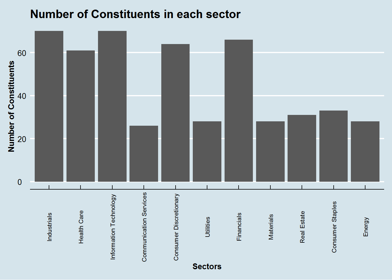

From the above chart we can quickly learn that Information Technology and Communication Services together dominate todays markets. Energy sector on the other hand has fewer constituents than Real Estate sector.