Scraping dataroma.com
An import task for many investors is to keep up with what other prominent investors are buying or selling. Such information is not very easily available. One needs to check the 13F filings and parse the data out. Fortunately, there are several websites that display such data in a nice tabular format.
One such website is https://www.dataroma.com.
This website lists the updated portfolio of many prominent investors. In this post we will try to get the data for Warren Buffett’s portfolio.
Get data for all investors
Lets start.
First we will load the libraries.
library(rvest)
library(tidyverse)
library(lubridate)
Next we will get the webpage we are interested in.
url <- "https://www.dataroma.com/m/home.php"
# Read the html page
url <- read_html(url)
We will check to see if the webpage was correctly downloaded.
print(url)## {xml_document}
## <html xmlns="http://www.w3.org/1999/xhtml" lang="en">
## [1] <head>\n<meta http-equiv="Content-Type" content="text/html; charset=UTF-8 ...
## [2] <body>\n<div id="mb">\n<div id="logo" unselectable="on">\nDATAROMA\n</div ...This page contains a lot of html information that is not useful for us. We are interested in the the names of all the investors and the urls that lead us to their portfolios.
So lets just parse our the relevant data. We will also print the first few names.
investor_names <- url %>%
  html_nodes('#port_body li') %>%
  html_text()

investor_names[1:15]
## [1] "Thomas Gayner - Markel Asset Management Updated 07 Feb 2020 "
## [2] "William Von Mueffling - Cantillon Capital Management Updated 07 Feb 2020 "
## [3] "Kahn Brothers Advisors - Kahn Brothers Group Updated 27 Jan 2020 "
## [4] "Wallace Weitz - Weitz Value Updated 22 Jan 2020 "
## [5] "Tweedy Browne Co. - Tweedy Browne Value Updated 21 Jan 2020 "
## [6] "Guy Spier - Aquamarine Capital Updated 17 Jan 2020 "
## [7] "Sam Peters - ClearBridge Value Trust Updated 16 Jan 2020 "
## [8] "Dodge & Cox Updated 15 Jan 2020 "
## [9] "Richard Pzena - Hancock Classic Value Updated 15 Jan 2020 "
## [10] "Mairs & Power - Mairs & Power Growth Updated 15 Jan 2020 "
## [11] "Steven Romick - FPA Crescent Fund Updated 13 Jan 2020 "
## [12] "FPA - Capital Fund Updated 13 Jan 2020 "
## [13] "Mark Hillman - Hillman Fund Updated 10 Jan 2020 "
## [14] "John Rogers - Ariel Appreciation Updated 08 Jan 2020 "
## [15] "Charles Bobrinskoy - Ariel Focus Updated 08 Jan 2020 "As expected we have the investor/fund names. Next lets get the relevant url for all the investors.
investor_url <- url %>%
  html_nodes('#port_body a') %>%
  html_attr("href")

investor_url[1:15]
## [1] "/m/holdings.php?m=MKL" "/m/holdings.php?m=cc"
## [3] "/m/holdings.php?m=KB" "/m/holdings.php?m=WVALX"
## [5] "/m/holdings.php?m=TWEBX" "/m/holdings.php?m=aq"
## [7] "/m/holdings.php?m=lmvtx" "/m/holdings.php?m=DODGX"
## [9] "/m/holdings.php?m=pzfvx" "/m/holdings.php?m=MPGFX"
## [11] "/m/holdings.php?m=FPACX" "/m/holdings.php?m=FPPTX"
## [13] "/m/holdings.php?m=hcmax" "/m/holdings.php?m=CAAPX"
## [15] "/m/holdings.php?m=ARFFX"This looks good. We now have both the Manager names and the url. Lets combine them into a nice table/dataframe.
investor_df <- tibble(investor = investor_names,
                      url = investor_url)
head(investor_df)
## # A tibble: 6 x 2
## investor url
## <chr> <chr>
## 1 "Thomas Gayner - Markel Asset Management Updated 07 Feb 2~ /m/holdings.php?m~
## 2 "William Von Mueffling - Cantillon Capital Management Upd~ /m/holdings.php?m~
## 3 "Kahn Brothers Advisors - Kahn Brothers Group Updated 27 ~ /m/holdings.php?m~
## 4 "Wallace Weitz - Weitz Value Updated 22 Jan 2020 " /m/holdings.php?m~
## 5 "Tweedy Browne Co. - Tweedy Browne Value Updated 21 Jan 2~ /m/holdings.php?m~
## 6 "Guy Spier - Aquamarine Capital Updated 17 Jan 2020 " /m/holdings.php?m~Next lets separate the investor column into two. We want to remove the Updated xxxx and form the investor name and move to a separate column. So we will end with two columns with the name and the date updated.
We will also add the https://www.dataroma.com to the url column.
investor_df <- investor_df %>%
  separate(investor,into = c('investor', 'update_date'), sep = 'Updated') %>%
  mutate_all(.funs = str_trim) %>%
  mutate(update_date = dmy(update_date)) %>%
  mutate(url = str_c('https://www.dataroma.com', url))

head(investor_df)
## # A tibble: 6 x 3
## investor update_date url
## <chr> <date> <chr>
## 1 Thomas Gayner - Markel Asset Manag~ 2020-02-07 https://www.dataroma.com/m/h~
## 2 William Von Mueffling - Cantillon ~ 2020-02-07 https://www.dataroma.com/m/h~
## 3 Kahn Brothers Advisors - Kahn Brot~ 2020-01-27 https://www.dataroma.com/m/h~
## 4 Wallace Weitz - Weitz Value 2020-01-22 https://www.dataroma.com/m/h~
## 5 Tweedy Browne Co. - Tweedy Browne ~ 2020-01-21 https://www.dataroma.com/m/h~
## 6 Guy Spier - Aquamarine Capital 2020-01-17 https://www.dataroma.com/m/h~It looks like our dataframe is complete. Now on to the next task to get Warren Buffett’s portfolio. We need to first select the link to Warren Buffetts’s portfolio. So lets see how we can do that.
Getting data for a specific investor
investor_df %>%
  filter(str_detect(investor,pattern = 'Warren'))
## # A tibble: 1 x 3
## investor update_date url
## <chr> <date> <chr>
## 1 Warren Buffett - Berkshire H~ 2019-11-14 https://www.dataroma.com/m/holding~We now have the row with Warren Buffett’s information.
Next just select the url and get his portfolio information.
warren_url <- investor_df %>%
  filter(str_detect(investor,pattern = 'Warren')) %>%
  select(url) %>%
  .[[1]]

print(warren_url)
## [1] "https://www.dataroma.com/m/holdings.php?m=BRK"Great, we have the correct url for the portfolio. Next we will repeat the above scraping process to get his portfolio. We will first store the text in a place holder variable called text. Next we will convert that into a dataframe.
warren_url <- read_html(warren_url)

# First store all the data in the 'text' variable

text <- warren_url %>%
  html_nodes('#grid td') %>%
  html_text()
Now lets see the first few values of the text variable and also the length of the variable.
text[1:30]## [1] "History" "Stock"
## [3] "% of portfolio" "Shares"
## [5] "Recent activity" "Reported Price*"
## [7] "Value" "="
## [9] "AAPL - Apple Inc." "25.96"
## [11] "248,838,679" "Reduce 0.30%"
## [13] "$223.97" "$55,732,400,000"
## [15] "=" "BAC - Bank of America Corp."
## [17] "12.60" "927,248,600"
## [19] " " "$29.17"
## [21] "$27,047,843,000" "="
## [23] "KO - Coca Cola Co." "10.14"
## [25] "400,000,000" " "
## [27] "$54.44" "$21,776,000,000"
## [29] "=" "WFC - Wells Fargo"length(text)## [1] 343We can see that the length of the text variable is 343 and we have the data that we were looking for. Next we will convert this 343 length vector into a table of 7 columns and 343/7 or 49 rows
# load the timetk library
library(timetk)
# First create a matrix

warren_mat <- matrix(text, ncol = 7, byrow = TRUE)

warren_df <- as.data.frame(warren_mat, stringsAsFactors = FALSE)

warren_df <- tk_tbl(warren_df, silent = TRUE)

warren_df
## # A tibble: 49 x 7
## V1 V2 V3 V4 V5 V6 V7
## <chr> <chr> <chr> <chr> <chr> <chr> <chr>
## 1 History Stock % of por~ Shares Recent ac~ Reported ~ Value
## 2 = AAPL - Apple In~ 25.96 248,838~ Reduce 0.~ $223.97 $55,732,4~
## 3 = BAC - Bank of A~ 12.60 927,248~ " " $29.17 $27,047,8~
## 4 = KO - Coca Cola ~ 10.14 400,000~ " " $54.44 $21,776,0~
## 5 = WFC - Wells Far~ 8.89 378,369~ Reduce 7.~ $50.44 $19,084,9~
## 6 = AXP - American ~ 8.35 151,610~ " " $118.28 $17,932,5~
## 7 = KHC - Kraft Hei~ 4.24 325,634~ " " $27.94 $9,096,60~
## 8 = USB - U.S. Banc~ 3.41 132,459~ " " $55.34 $7,330,31~
## 9 = JPM - JPMorgan ~ 3.26 59,514,~ " " $117.69 $7,004,31~
## 10 = MCO - Moody's C~ 2.35 24,669,~ " " $204.83 $5,053,11~
## # ... with 39 more rowsWe have successfully downloaded the data. Next we need to do some cleanup.
We will do the following.
- Use the first row as column names
- Delete the first row
- Delete the unnecessary columns
- Change the column names
- Separate the
stockcolumn intosymbolandname - Convert the numbers into percent and remove the
$and,sign from columns
So lets do it.
# Change column names
colnames(warren_df) <- warren_df[1,]

# Delete the first row
warren_df <- warren_df[-1,]

warren_df <- warren_df %>%
  select(-c(History,`Recent activity`)) %>%
  `colnames<-`(c('stock','portfolio_weight', 'shares','cost_price', 'value')) %>%
  separate(stock, into = c('symbol', 'name'), sep = '-') %>%
  mutate_all(.funs = str_trim) %>%
  mutate_at(.vars = c('shares','cost_price','value'), .funs = parse_number) %>%
  mutate(portfolio_weight = parse_number(portfolio_weight)/100)

warren_df
## # A tibble: 48 x 6
## symbol name portfolio_weight shares cost_price value
## <chr> <chr> <dbl> <dbl> <dbl> <dbl>
## 1 AAPL Apple Inc. 0.260 248838679 224. 5.57e10
## 2 BAC Bank of America Cor~ 0.126 927248600 29.2 2.70e10
## 3 KO Coca Cola Co. 0.101 400000000 54.4 2.18e10
## 4 WFC Wells Fargo 0.0889 378369018 50.4 1.91e10
## 5 AXP American Express 0.0835 151610700 118. 1.79e10
## 6 KHC Kraft Heinz Co. 0.0424 325634818 27.9 9.10e 9
## 7 USB U.S. Bancorp 0.0341 132459618 55.3 7.33e 9
## 8 JPM JPMorgan Chase & Co. 0.0326 59514932 118. 7.00e 9
## 9 MCO Moody's Corp. 0.0235 24669778 205. 5.05e 9
## 10 DAL Delta Air Lines Inc. 0.019 70910456 57.6 4.08e 9
## # ... with 38 more rowsWe now have the table in the desired form. We can now use it for our analysis.
What about other investors?
But a thought may pop in your head, that this is a lot of work and what if we need to download the data for another investor. Do we repeat this process again?
No. We do not need to repeat this process again, if we build a function to do this for us automatically.
So lets do that. We will build two functions. First gets the Names and urls of all the investors. The second gets the portfolio of the investor we are interested in.
So lets build our first function
get_all_investors <- function() {

  library(rvest)
  library(lubridate)
  library(tidyverse)

  url <- "https://www.dataroma.com/m/home.php"
  # Read the html page
  url <- read_html(url)

  # Get the investor names
  investor_names <- url %>%
    html_nodes('#port_body li') %>%
    html_text()

  # Get the investor url

  investor_url <- url %>%
    html_nodes('#port_body a') %>%
    html_attr("href")

  # Build the dataframe

  investor_df <- tibble(investor = investor_names,
                        url = investor_url)


  # Cleanup the table

  investor_df <- investor_df %>%
    separate(investor,into = c('investor', 'update_date'), sep = 'Updated') %>%
    mutate_all(.funs = str_trim) %>%
    mutate(update_date = dmy(update_date)) %>%
    mutate(url = str_c('https://www.dataroma.com', url))

  # Return the values
  return(investor_df)
}
Lets test it.
all_investors <- get_all_investors()

all_investors
## # A tibble: 64 x 3
## investor update_date url
## <chr> <date> <chr>
## 1 Thomas Gayner - Markel Asset Mana~ 2020-02-07 https://www.dataroma.com/m/h~
## 2 William Von Mueffling - Cantillon~ 2020-02-07 https://www.dataroma.com/m/h~
## 3 Kahn Brothers Advisors - Kahn Bro~ 2020-01-27 https://www.dataroma.com/m/h~
## 4 Wallace Weitz - Weitz Value 2020-01-22 https://www.dataroma.com/m/h~
## 5 Tweedy Browne Co. - Tweedy Browne~ 2020-01-21 https://www.dataroma.com/m/h~
## 6 Guy Spier - Aquamarine Capital 2020-01-17 https://www.dataroma.com/m/h~
## 7 Sam Peters - ClearBridge Value Tr~ 2020-01-16 https://www.dataroma.com/m/h~
## 8 Dodge & Cox 2020-01-15 https://www.dataroma.com/m/h~
## 9 Richard Pzena - Hancock Classic V~ 2020-01-15 https://www.dataroma.com/m/h~
## 10 Mairs & Power - Mairs & Power Gro~ 2020-01-15 https://www.dataroma.com/m/h~
## # ... with 54 more rowsGreat that function works. Next we build our portfolio function.
get_investor_portfolio <- function(name = 'Warren') {

  # First get all the investors
  all_investors <- get_all_investors()

  # Sometime users can type a lower case name
  name = str_to_lower(name)
  name = str_to_title(name)

  # This is to catch any errors
  tryCatch(

    expr = {

      # Get specific url
      url <- all_investors %>%
        filter(str_detect(investor,pattern = name)) %>%
        select(url) %>%
        .[[1]]

      # Read the html

      url <- read_html(url)
    # get the data into 'text' variable

      text <- url %>%
        html_nodes('#grid td') %>%
        html_text()

  # Load timetk for table conversion
  library(timetk)

  # First create a matrix
  investor_mat <- matrix(text, ncol = 7, byrow = TRUE)

  # Convert to data frame
  investor_df <- as.data.frame(investor_mat, stringsAsFactors = FALSE)

  # Convert to tibble
  investor_df <- tk_tbl(investor_df, silent = TRUE)

  # Change column names
  colnames(investor_df) <- investor_df[1,]

  # Delete the first row
  investor_df <- investor_df[-1,]

  # Final Table
  investor_df <- investor_df %>%
    select(-c(History,`Recent activity`)) %>%
    `colnames<-`(c('stock','portfolio_weight', 'shares','cost_price', 'value')) %>%
    separate(stock, into = c('symbol', 'name'), sep = '-') %>%
    mutate_all(.funs = str_trim) %>%
    mutate_at(.vars = c('shares','cost_price','value'), .funs = parse_number) %>%
    mutate(portfolio_weight = parse_number(portfolio_weight)/100)

  # Return the table
  return(investor_df)

    },

  # Igonore this
  # This is execuated when we get an error
  error = function(e) {

    message('This investor does not exist. Make sure this investor is listed on the www.dataroma.com website')
    print(e)
  }

  )

}
That is a big function, but it will help us get any manager’s portfolio that is listed on the www.dataroma.com. So lets give it a try.
Lets try an get Bill Ackman’s portfolio
ackman <- get_investor_portfolio("Ackman")

ackman
## # A tibble: 8 x 6
## symbol name portfolio_weight shares cost_price value
## <chr> <chr> <dbl> <dbl> <dbl> <dbl>
## 1 CMG Chipotle Mexican Grill ~ 0.223 1724310 840. 1.45e9
## 2 QSR Restaurant Brands Inter~ 0.165 15084304 71.1 1.07e9
## 3 HLT Hilton Worldwide Holdin~ 0.152 10556805 93.1 9.83e8
## 4 LOW Lowe's Cos. 0.146 8613212 110. 9.47e8
## 5 BRK.B Berkshire Hathaway CL B 0.129 4015594 208. 8.35e8
## 6 SBUX Starbucks Corp. 0.127 9313890 88.4 8.24e8
## 7 A Agilent Technologies 0.0344 2916103 76.6 2.23e8
## 8 HHC Howard Hughes Corp. 0.0239 1194793 130. 1.55e8And now we can plot Ackman’s Portfolio.
# For themes
library(ggthemes)

ackman %>%
  ggplot(aes(x = fct_reorder(factor(symbol),portfolio_weight), y = portfolio_weight)) +
  geom_bar(stat = 'identity') +
  labs(x = 'Symbol',
       y = 'Portfolio Weight', title = 'Bill Ackmans Portfolio Holdings') +
  theme_fivethirtyeight() +
  scale_y_continuous(labels = scales::percent)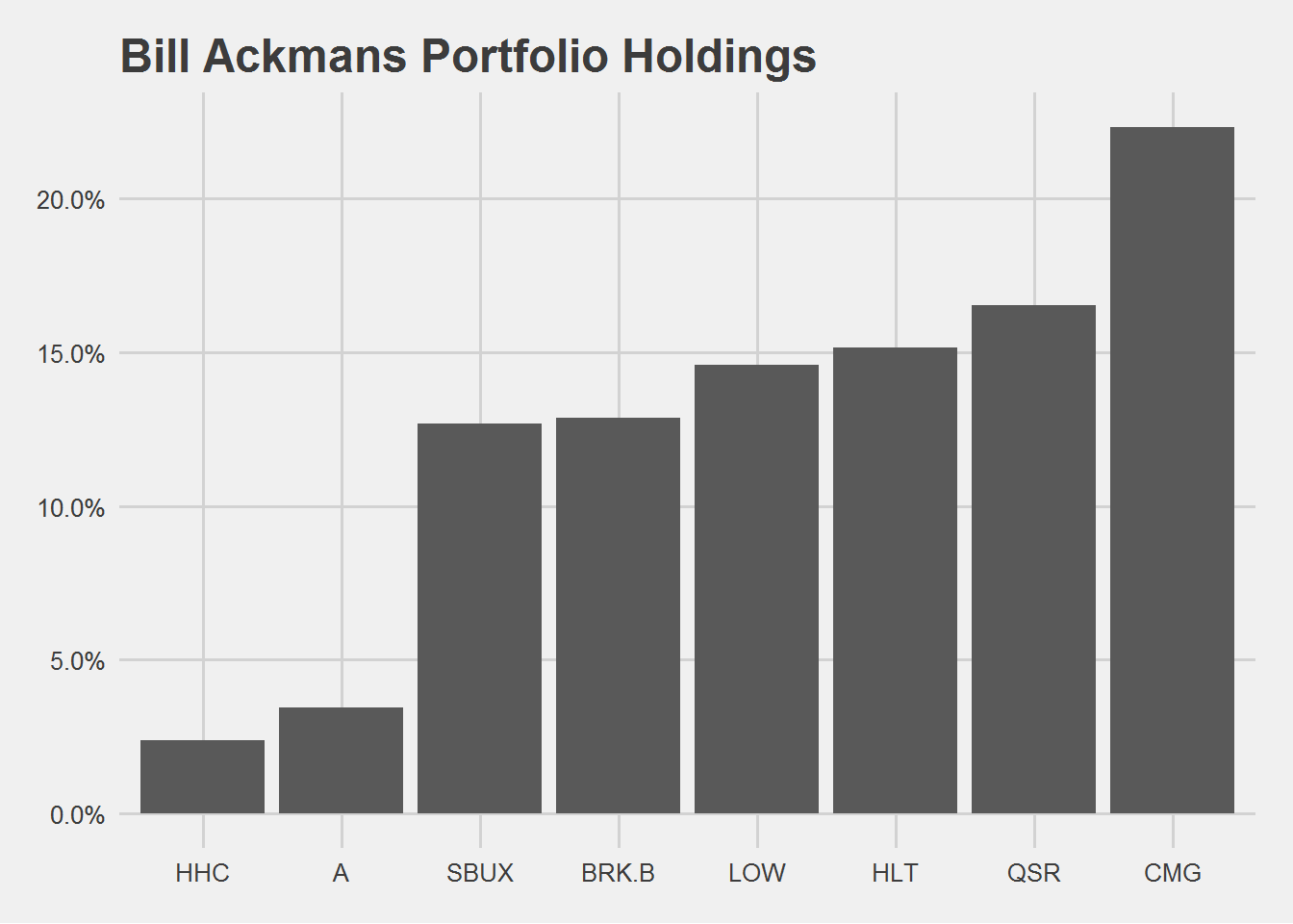
Lets try one more investor - Daniel Loeb.
loeb <- get_investor_portfolio('Loeb')

loeb
## # A tibble: 39 x 6
## symbol name portfolio_weight shares cost_price value
## <chr> <chr> <dbl> <dbl> <dbl> <dbl>
## 1 BAX Baxter International In~ 0.175 1.68e7 87.5 1.47e9
## 2 UTX United Technologies 0.0974 6.00e6 137. 8.19e8
## 3 CPB Campbell Soup 0.0948 1.70e7 46.9 7.98e8
## 4 AGN Allergan Plc 0.072 3.60e6 168. 6.06e8
## 5 DHR Danaher Corp. 0.0637 3.71e6 144. 5.36e8
## 6 BID Sotheby's 0.0451 6.66e6 57.0 3.80e8
## 7 CRM Salesforce.com 0.0441 2.50e6 148. 3.71e8
## 8 FIS Fidelity National Infor~ 0.0394 2.50e6 133. 3.32e8
## 9 BURL Burlington Stores Inc. 0.0356 1.50e6 200. 3.00e8
## 10 IQV IQVIA Holdings Inc. 0.0355 2.00e6 149. 2.99e8
## # ... with 29 more rowsCompared to Bill Ackman, Loeb’s portfolio contains more positions. We will only look at positions above 2% weight.
loeb %>%
  filter(portfolio_weight > 0.02) %>%
  ggplot(aes(x = fct_reorder(factor(symbol),portfolio_weight), y = portfolio_weight)) +
  geom_bar(stat = 'identity') +
  labs(x = 'Symbol',
       y = 'Portfolio Weight', title = 'Daniel Loeb\'s Portfolio Holdings') +
  theme_fivethirtyeight() +
  scale_y_continuous(labels = scales::percent,
                     breaks = seq(0,0.25,0.03))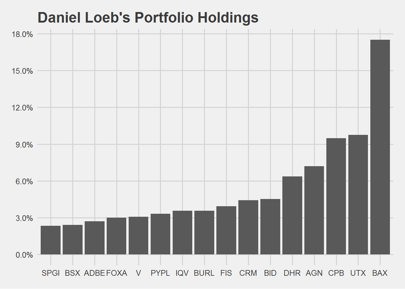
That’s it. We have successfully automated our function to get portfolio data from the internet. We use this data to plot a simple portfolio position chart.