Quantitative Investment Analysis - Chapter 6
library(tidyverse)
library(knitr)
library(kableExtra)
In this post we will solve the end of the chapter practice problems from chapter 6 of the book.
Problem 1
Peter Biggs wants to know how growth managers performed last year. Biggs assumes that the population cross-sectional standard deviation of growth manager returns is 6 percent and that the returns are independent across managers.
- A How large a random sample does Biggs need if he wants the standard deviation of the sample means to be 1 percent?
- B How large a random sample does Biggs need if he wants the standard deviation of the sample means to be 0.25 percent?
We know that

# Population sd is 0.06
pop_sd <- 6/100

# The standard deviation or standard error of the sample mean is σX = σ / sqrt(n)
# 0.01 = pop_sd / sqrt(n)

n = (pop_sd / 0.01) ** 2

cat("Biggs need", n, "samples, if he wants the standard deviation
    of the sample means to be 1 percent")
## Biggs need 36 samples, if he wants the standard deviation
## of the sample means to be 1 percentA - Biggs need 36 samples, if he wants the standard deviation of the sample means to be 1 percent
n = (pop_sd / 0.0025) ** 2

cat("Biggs need", n, "samples, if he wants the standard deviation
    of the sample means to be 0.25 percent")
## Biggs need 576 samples, if he wants the standard deviation
## of the sample means to be 0.25 percentB - Biggs need 576 samples, if he wants the standard deviation of the sample means to be 0.25 percent
As standard error decreases, the sample size increases.
Problem 2
Petra Munzi wants to know how value managers performed last year. Munzi estimates that the population cross-sectional standard deviation of value manager returns is 4 percent and assumes that the returns are independent across managers.
- A Munzi wants to build a 95 percent confidence interval for the mean return. How large a random sample does Munzi need if she wants the 95 percent confidence interval to have a total width of 1 percent?
- B Munzi expects a cost of about $10 to collect each observation. If she has a $1,000 budget, will she be able to construct the confidence interval she wants?
# We know population sd

pop_sd <- 0.04

# se is s/sqrt(n) # standard error
# we have to find n
# but before that we need to find se
# 95% confidence interval means
# 2.5% in each tail

lower_tail <- qnorm(0.025, lower.tail = T)
uppper_tail <- qnorm(0.025, lower.tail = F)

cat("lower tail", lower_tail,"\n",
    "upper tail", uppper_tail)
## lower tail -1.959964
## upper tail 1.959964So we need our 95% confidence interval to have a 1% width.
# Assuming X as our mean and se as our sample sd
# We have (X + 1.96se) − (X − 1.96se) = 1%
# which is equal to 2*(1.96se) = 1%
# se = 0.01 / (2 * 1.96)

se <- 0.01 / (2 * uppper_tail)
cat("The standard deviation of sample mean is,", se, "\n\n\n")
## The standard deviation of sample mean is, 0.002551067# Now find the n
n <- (0.04 / se) ** 2
cat("Munzi needs a sample size of", round(n), "if she wants the 95 percent
confidence interval to have a total width of 1 percent")## Munzi needs a sample size of 246 if she wants the 95 percent
## confidence interval to have a total width of 1 percentA - Munzi needs a sample size of 246 if she wants the 95 percent confidence interval to have a total width of 1 percent
B - With her $1000 budget Munzi can only afford 100 observations which is far short of 246 she needs to have a 1% width of her confidence interval.
Problem 3
Assume that the equity risk premium is normally distributed with a population mean of 6 percent and a population standard deviation of 18 percent. Over the last four years, equity returns (relative to the risk-free rate) have averaged −2.0 percent. You have a large client who is very upset and claims that results this poor should never occur. Evaluate your client’s concerns.
- A Construct a 95 percent confidence interval around the population mean for a sample of four-year returns.
- B What is the probability of a −2.0 percent or lower average return over a four-year period?
# Assuming normal distribution
# Pop mean
m <- 6/100

# Pop sd
s <- 18/100

# we need the se for last 4 years
# se is the sample sd
# se = sd / sqrt(4)

se <- s / sqrt(4)

# 95% confidence interval will
# have 2.5% in each tail

# upper limit
upper_limit <- qnorm(0.025, m, se,lower.tail = F)

# lower limit

lower_limit <- qnorm(0.025, m, se,lower.tail = T)

cat( "A 95 percent confidence interval around the population mean for
a sample of four-year
returns has upper limit of",
upper_limit, "and a lower limit of", lower_limit)
## A 95 percent confidence interval around the population mean for
## a sample of four-year
## returns has upper limit of 0.2363968 and a lower limit of -0.1163968A - There is a 95% probability that returns will fall between ~23.7% and ~-11.64%
# lower limit is -2%

# Probability of getting
# -2% or lower returns over a 4 year period is

p <- pnorm(-0.02,mean = m, sd = se, lower.tail = T)

cat("The probability of a −2.0 percent or lower average return over a
four-year
period is", p)
## The probability of a −2.0 percent or lower average return over a
## four-year
## period is 0.1870314B- The probability of a −2.0 percent or lower average return over a four-year period is 0.1870314
Problem 4
Compare the standard normal distribution and Student’s t-distribution.
See below plots for comparison
x <- seq(-4,4,length = 1000)

# normal distribution
d_x <- dnorm(x)

# df = degrees of freedom
# t distribution with 2 df
d_x1 <- dt(x, 2)

# t distribution with 5 df
d_x2 <- dt(x, 5)

# make our tibble
# plot the chart

tibble(x = x,
       d_x = d_x,
       d_x1 = d_x1,
       d_x2 = d_x2) %>%
  ggplot(aes(x = x, y = d_x, color = 'normal\ndistribution')) +
  geom_line() +
  geom_line(aes(x = x, y = d_x1, color = 't with\ndf = 2')) +
  geom_line(aes(x = x, y = d_x2, color = 't with\ndf = 5')) +
  labs(x = 'x',
       y = 'f(x)',
       title = 'Comparing Normal Distribution with t distribution') +
  scale_colour_discrete("Distributions") +
  theme_classic() +
  scale_y_continuous(expand = c(0,0))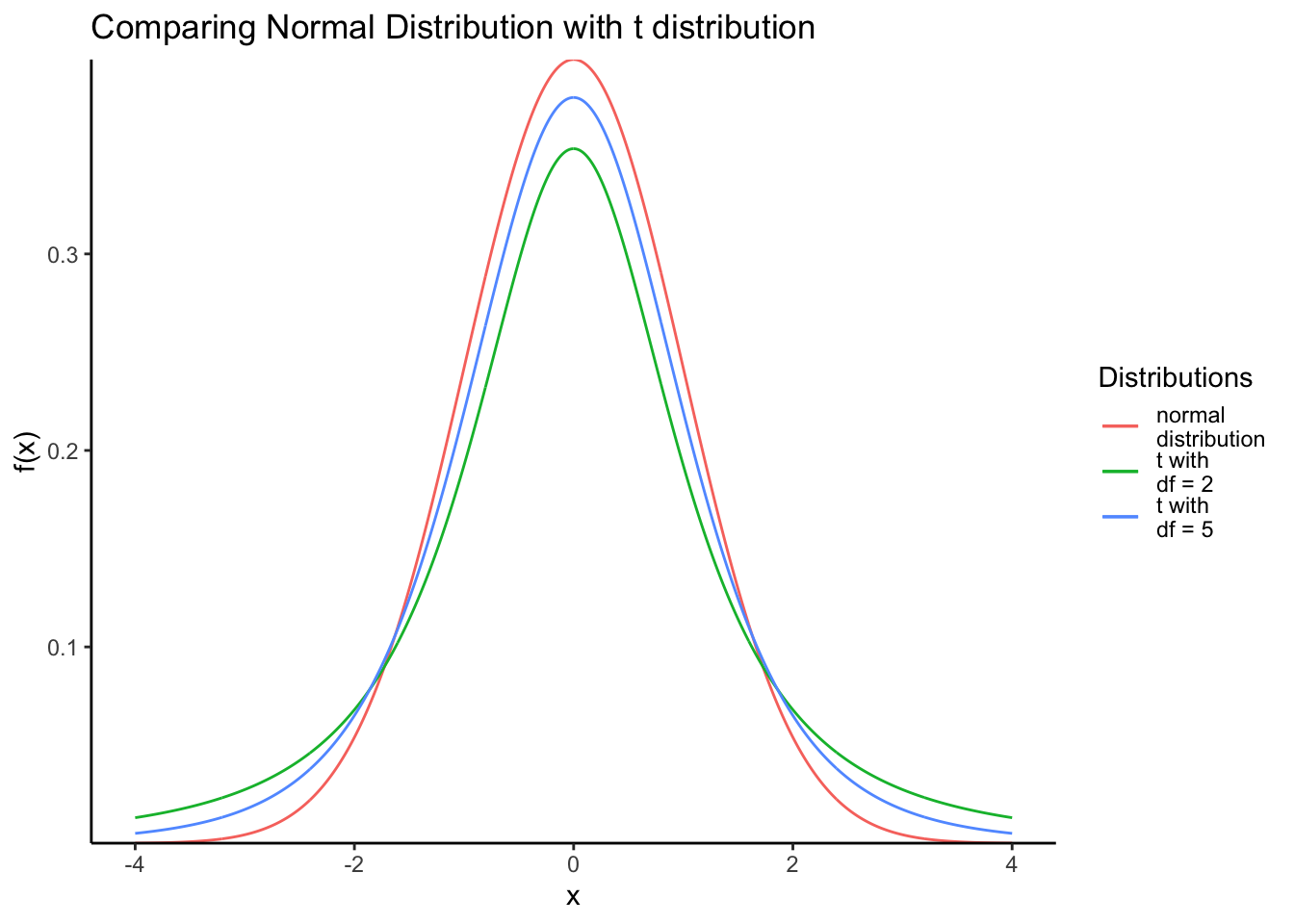
Problem 5
Find the reliability factors based on the t-distribution for the following confidence intervals for the population mean (df = degrees of freedom, n = sample size):
- A A 99 percent confidence interval, df = 20.
- B A 90 percent confidence interval, df = 20.
- C A 95 percent confidence interval, n = 25.
- D A 95 percent confidence interval, n = 16
# As we did in Problem 4
# we will use the t() functions

# 99% with df = 20

level <- (1 - 0.99)/2
df <- 20

f1 <- qt(level, df = df, lower.tail = F)

cat("A 99 percent confidence interval, df = 20 is", f1)
## A 99 percent confidence interval, df = 20 is 2.84534A - A 99 percent confidence interval, df = 20 is 2.84534
# 90% with df = 20

level <- (1 - 0.90)/2
df <- 20

f1 <- qt(level, df = df, lower.tail = F)

cat("A 90 percent confidence interval, df = 20 is", f1)
## A 90 percent confidence interval, df = 20 is 1.724718B - A 90 percent confidence interval, df = 20 is 1.724718
# 95% with n = 25
# df = n - 1

n = 25
df <- n - 1

level <- (1 - 0.95)/2

f1 <- qt(level, df = df, lower.tail = F)

cat("A 95 percent confidence interval, n = 25 is", f1)
## A 95 percent confidence interval, n = 25 is 2.063899C - A 95 percent confidence interval, df = 25 is 2.063899
# 95% with n = 16
# df = n - 1

n = 16
df <- n - 1

level <- (1 - 0.95)/2

f1 <- qt(level, df = df, lower.tail = F)

cat("A 95 percent confidence interval, n = 16 is", f1)
## A 95 percent confidence interval, n = 16 is 2.13145D - A 95 percent confidence interval, n = 16 is 2.13145
Problem 6
Assume that monthly returns are normally distributed with a mean of 1 percent and a sample standard deviation of 4 percent. The population standard deviation is unknown. Construct a 95 percent confidence interval for the sample mean of monthly returns if the sample size is 24.
# pop mean
m <- 1/100
# sd
s <- 4/100

# sample
n <- 24
df <- n - 1

# 95% conf interval

level <- (1 - 0.95) / 2

# Calculate the se

error <- qt(level, df = df, lower.tail = F) * (s / sqrt(n))

upper <- m + error
lower <- m - error

cat("A 95 percent confidence interval will fall between", lower, "and", upper)
## A 95 percent confidence interval will fall between -0.006890519 and 0.02689052A 95% confidence interval will fall between -0.006890519 and 0.02689052
Problem 7
Ten analysts have given the following fiscal year earnings forecasts for a stock:
| Forecast | Number of Analysts |
|---|---|
| 1.40 | 1 |
| 1.43 | 1 |
| 1.44 | 3 |
| 1.45 | 2 |
| 1.47 | 1 |
| 1.48 | 1 |
| 1.50 | 1 |
Because the sample is a small fraction of the number of analysts who follow this stock, assume that we can ignore the finite population correction factor. Assume that the analyst forecasts are normally distributed.
- A What are the mean forecast and standard deviation of forecasts?
- B Provide a 95 percent confidence interval for the population mean of the forecasts.
# Forecast
f <- c(1.4,1.43,1.44,1.45,1.47,1.48,1.5)

# number of analysts
n <- c(1,1,3,2,1,1,1)

# total analyst
num <- sum(n)

# calculate weights
w <- n / sum(n)

# Weighted Mean
m <- weighted.mean(f, w)

cat("Mean Forecast is", m)
## Mean Forecast is 1.45cat("\n")# Standard Deviation
v <- sum(n * (f - m) ** 2) / (num - 1)
s <- sqrt(v)
cat("Standard Deviation is", s)## Standard Deviation is 0.02788867A - Mean Forecast is 1.45 and the Standard Deviation is 0.02788867
# 95% confidence Interval

level <- (1 - 0.95) / 2
df <- num - 1


error <- qt(level,df = df,
            lower.tail = F) * (s/sqrt(10))

upper <- m + error
lower <- m - error

cat("Upper and Lower limits are", upper,'\n', lower)
## Upper and Lower limits are 1.46995
## 1.43005Upper and Lower limits are 1.46995 and 1.43005
Problem 8
Thirteen analysts have given the following fiscal-year earnings forecasts for a stock
| Forecast | Number of Analyst |
|---|---|
| 0.70 | 2 |
| 0.72 | 4 |
| 0.74 | 1 |
| 0.75 | 3 |
| 0.76 | 1 |
| 0.77 | 1 |
| 0.82 | 1 |
Because the sample is a small fraction of the number of analysts who follow this stock, assume that we can ignore the finite population correction factor.
- A What are the mean forecast and standard deviation of forecasts?
- B What aspect of the data makes us uncomfortable about using t-tables to construct confidence intervals for the population mean forecast?
# Forecasts
f <- c(0.7,0.72,0.74, 0.75,0.76,0.77,0.82)

# number of analyst
n <- c(2,4,1,3,1,1,1)

# Total analyst
num <- sum(n)

# weights of each forecast
w <- n / sum(n)

# Calculate the weighted mean
m <- weighted.mean(f,w)

# Calculate the SD
# variance
v <- sum(((f - m)^2) * n) / (num - 1)

# SD

s <- sqrt(v)


cat("The mean forecast is,", m, "and the standard deviation of forecast is,",s)
## The mean forecast is, 0.74 and the standard deviation of forecast is, 0.03265986A - The mean forecast is, 0.74 and the standard deviation of forecast is, 0.03265986
# Get the forecast from all analysts
x <- rep(f,n)

# plot the histogram of the forecast

ggplot(aes(x = x), data = NULL) +
  geom_histogram(bins = 50)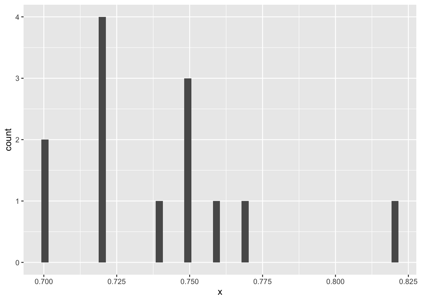
B - The sample is small, and the distribution of the forecast appear to be bimodal, and we cannot compute the confidence intervals as the distribution appears to be not normal.
Problem 9
Explain the differences between constructing a confidence interval when sampling from a normal population with a known population variance and sampling from a normal population with an unknown variance
For a known standard deviation: we use the formula

For an unknown standard deviation we use the formula

Problem 10
An exchange rate has a given expected future value and standard deviation.
- A Assuming that the exchange rate is normally distributed, what are the probabilities that the exchange rate will be at least 2 or 3 standard deviations away from its mean?
- B Assume that you do not know the distribution of exchange rates. Use Chebyshev’s inequality (that at least 1 − 1/k2 proportion of the observations will be within k standard deviations of the mean for any positive integer k greater than 1) to calculate the maximum probabilities that the exchange rate will be at least 2 or 3 standard deviations away from its mean.
# We know the z value

# When z is 2

z_2 <- (1 - pnorm(2)) * 2

# When z is 3

z_3 <- (1 - pnorm(3)) * 2

cat("The probability that the exchange rate will be at least 2 standard deviations away from the mean is", z_2, "and 3 standard deviations away from the mean is", z_3)
## The probability that the exchange rate will be at least 2 standard deviations away from the mean is 0.04550026 and 3 standard deviations away from the mean is 0.002699796A - The probability that the exchange rate will be at least 2 standard deviations away from the mean is 0.04550026 and 3 standard deviations away from the mean is 0.002699796
# Since the distribution is unknown and using Chevychev's theorem

# when k = 2

k_2 <- (1 - (1/2)^2)

# when k = 3
k_3 <- (1 - (1/3)^2)

cat("The maximum probabilities that the exchange
rate will be at least 2 standard deviations away from its mean is", 1 - k_2,
"or 3 standard deviations away from its mean is", 1- k_3)
## The maximum probabilities that the exchange
## rate will be at least 2 standard deviations away from its mean is 0.25 or 3 standard deviations away from its mean is 0.1111111We can see that when the distribution is unknown and using Chebychev’s theorem, the probabilities of getting extreme data increases.
Problem 11
Although he knows security returns are not independent, a colleague makes the claim that because of the central limit theorem, if we diversify across a large number of investments, the portfolio standard deviation will eventually approach zero as n becomes large. Is he correct?
As we increase the number of securities, the standard deviation will get lower but not approach zero. This has nothing to do with the central limit theorem, but due to correlation of different assets.
Problem 12
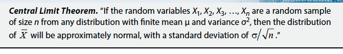
Why is the central limit theorem important?
Please watch these excellent videos
Links for the video(in case they don’t show up in your browser)
Problem 13
What is wrong with the following statement of the central limit theorem?
- First the sample size
nhas to be large (above 30) - The distribution will have a mean approximately equal to population mean
Problem 14
Suppose we take a random sample of 30 companies in an industry with 200 companies. We calculate the sample mean of the ratio of cash flow to total debt for the prior year. We find that this ratio is 23 percent. Subsequently, we learn that the population cash flow to total debt ratio (taking account of all 200 companies) is 26 percent. What is the explanation for the discrepancy between the sample mean of 23 percent and the population mean of 26 percent?
- A Sampling error.
- B Bias.
- C A lack of consistency.
A Sampling error
Problem 15
Alcorn Mutual Funds is placing large advertisements in several financial publications. The advertisements prominently display the returns of 5 of Alcorn’s 30 funds for the past 1-, 3-, 5-, and 10-year periods. The results are indeed impressive, with all of the funds beating the major market indexes and a few beating them by a large margin. Is the Alcorn family of funds superior to its competitors?
Selecting only 5 out of 30 funds may indicate selection bias. We will have to analyze the performance of all the funds to come to a conclusion if Alcorn family of funds is superior to its competitors.
Problem 16
Julius Spence has tested several predictive models in order to identify undervalued stocks. Spence used about 30 company-specific variables and 10 market-related variables to predict returns for about 5,000 North American and European stocks. He found that a final model using eight variables applied to telecommunications and computer stocks yields spectacular results. Spence wants you to use the model to select investments. Should you? What steps would you take to evaluate the model?
If you test so many variables, there is a high probability that some variables will be statistically significant. It would have been surprising, if there were no varibales that yielded spectacular results.
To test the model we should question the models and make sure it makes economic sense. We should also split the data and test the model on an out of sample data.
Probllem 17
The best approach for creating a stratified random sample of a population involves:
- A drawing an equal number of simple random samples from each subpopulation.
- B selecting every kth member of the population until the desired sample size is reached.
- C drawing simple random samples from each subpopulation in sizes proportional to the relative size of each subpopulation
C drawing simple random samples from each subpopulation in sizes proportional to the relative size of each subpopulation
Problem 18
A population has a non-normal distribution with mean μ and variance σ2. The sampling distribution of the sample mean computed from samples of large size from that population will have:
- A the same distribution as the population distribution.
- B its mean approximately equal to the population mean.
- C its variance approximately equal to the population variance.
B its mean approximately equal to the population mean.
Problem 19
A sample mean is computed from a population with a variance of 2.45. The sample size is 40. The standard error of the sample mean is closest to:
- A 0.039.
- B 0.247.
- C 0.387.
# pop variance
v <- 2.45
s <- sqrt(v)

# size = 40
size <- 40

# se = standard error

se <- s / sqrt(size)

cat('The standard error of the sample mean is closest to:', se)
## The standard error of the sample mean is closest to: 0.2474874B 0.247
Problem 20
An estimator with an expected value equal to the parameter that it is intended to estimate is described as:
- A efficient.
- B unbiased.
- C consistent.
B unbiased
An unbiased estimator is one for which the expected value equals the parameter it is intended to estimate
Problem 21
If an estimator is consistent, an increase in sample size will increase the:
- A accuracy of estimates.
- B efficiency of the estimator.
- C unbiasedness of the estimator
A accuracy of estimates.
Problem 22
For a two-sided confidence interval, an increase in the degree of confidence will result in:
- A a wider confidence interval.
- B a narrower confidence interval.
- C no change in the width of the confidence interval.
A a wider confidence interval.
Problem 23
As the t-distribution’s degrees of freedom decrease, the t-distribution most likely:
- A exhibits tails that become fatter.
- B approaches a standard normal distribution.
- C becomes asymmetrically distributed around its mean value.
A exhibits tails that become fatter.
Problem 24
For a sample size of 17, with a mean of 116.23 and a variance of 245.55, the width of a 90% confidence interval using the appropriate t-distribution is closest to:
- A 13.23.
- B 13.27.
- C 13.68.
# mean
m <- 116.23

# variance
v <- 245.55

# sd
s <- sqrt(v)

# size
size <- 17

# alpha 0.1
a <- 0.1

# at 90% confidence interval and
# df = size - 1
t_a <- qt(a/2, df = size - 1, lower.tail = F)

error <- t_a * (s / sqrt(size))

upper <- m + error
lower <- m - error

interval <- upper - lower

cat("the width of a 90% confidence interval using the appropriate t-distribution is closest
to:", interval)
## the width of a 90% confidence interval using the appropriate t-distribution is closest
## to: 13.27061B 13.27
Problem 25
For a sample size of 65 with a mean of 31 taken from a normally distributed population with a variance of 529, a 99% confidence interval for the population mean will have a lower limit closest to:
- A 23.64.
- B 25.41.
- C 30.09.
# Normal Distribution
# size
size <- 65

# mean
m <- 31

# variance
v <- 529

# sd
s <- sqrt(v)

# alpha 0.01
a <- 0.01

# at 99% confidence interval and
# df of size - 1

t_a <- qnorm(a/2)

error <- t_a * (s / sqrt(size))

lower <- m + error
cat("A 99% confidence interval for the population
mean will have a lower limit closest to:", lower)
## A 99% confidence interval for the population
## mean will have a lower limit closest to: 23.65168A 23.65
Problem 26
An increase in sample size is most likely to result in a:
- A wider confidence interval.
- B decrease in the standard error of the sample mean.
- C lower likelihood of sampling from more than one population.
B decrease in the standard error of the sample mean.
Problem 27
A report on long-term stock returns focused exclusively on all currently publicly traded firms in an industry is most likely susceptible to:
- A look-ahead bias.
- B survivorship bias.
- C intergenerational data mining.
B survivorship bias.
Problem 28
Which sampling bias is most likely investigated with an out-of- sample test?
- A Look-ahead bias
- B Data-mining bias
- C Sample selection bias
C Sample selection bias
Problem 29
Which of the following characteristics of an investment study most likely indicates time-period bias?
- A The study is based on a short time-series.
- B Information not available on the test date is used.
- C A structural change occurred prior to the start of the study’s time series.
A The study is based on a short time-series.