Quantitative Investment Analysis - Chapter 7
library(tidyverse)
library(knitr)
library(kableExtra)
In this post we will solve the end of the chapter practice problems from chapter 7 of the book.
Problem 1
Which of the following statements about hypothesis testing is correct?
- A The null hypothesis is the condition a researcher hopes to support.
- B The alternative hypothesis is the proposition considered true without conclusive evidence to the contrary.
C The alternative hypothesis exhausts all potential parameter values not accounted for by the null hypothesis.
C The alternative hypothesis exhausts all potential parameter values not accounted for by the null hypothesis.
Problem 2
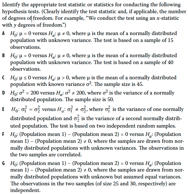
A - We conduct the t-test with (15 - 1) = 14 degrees of freedom.
B - We conduct the t-test with (40 - 1) = 39 degrees of freedom.
C - We conduct the z-statistic test since the sample comes from a normal distribution
D - We conduct the chi-square test with (50 -1) = 49 degress of freedom
E - We conduct the F-statistic test
F - We conduct the t-statistic test for a paired observation
G - We conduct a t-statistic test using a pooled estimate of population variance and (25 + 30 - 2) = 53 degrees of freedom
Problem 3
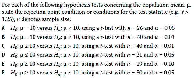
size <- 26

df <- size - 1

# alpha

a <- 0.05

upper <- qt(a/2,df = df, lower.tail = F)
lower <- qt(a/2,df = df)

cat("For significant level of", a, "the rejection values are greater than", upper, "and less than", lower)
## For significant level of 0.05 the rejection values are greater than 2.059539 and less than -2.059539A - For significant level of 0.05 the rejection values are greater than 2.059539 and less than -2.059539
size <- 40

df <- size - 1

# alpha

a <- 0.01

upper <- qt(a/2,df = df, lower.tail = F)
lower <- qt(a/2,df = df)

cat("For significant level of", a, "the rejection values are greater than", upper, "and less than", lower)
## For significant level of 0.01 the rejection values are greater than 2.707913 and less than -2.707913B - For significant level of 0.01 the rejection values are greater than 2.707913 and less than -2.707913
size <- 40

df <- size - 1

# alpha

a <- 0.01

upper <- qt(a,df = df, lower.tail = F)

cat("For significant level of", a, "the rejection values are greater than", upper)
## For significant level of 0.01 the rejection values are greater than 2.425841C - For significant level of 0.01 the rejection values are greater than 2.425841
size <- 21

df <- size - 1

# alpha

a <- 0.05

upper <- qt(a,df = df, lower.tail = F)

cat("For significant level of", a, "the rejection values are greater than", upper)
## For significant level of 0.05 the rejection values are greater than 1.724718D - For significant level of 0.05 the rejection values are greater than 1.724718
size <- 19

df <- size - 1

# alpha

a <- 0.1

lower <- qt(a,df = df)

cat("For significant level of", a, "the rejection values are less than", lower)
## For significant level of 0.1 the rejection values are less than -1.330391E - For significant level of 0.1 the rejection values are less than -1.330391
size <- 50

df <- size - 1

# alpha

a <- 0.05

lower <- qt(a,df = df)

cat("For significant level of", a, "the rejection values are less than", lower)
## For significant level of 0.05 the rejection values are less than -1.676551For significant level of 0.05 the rejection values are less than -1.676551
Problem 4
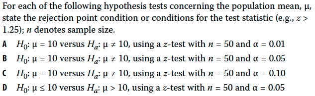
# alpha
a <- 0.01

upper <- qnorm(a/2, lower.tail = F)
lower <- qnorm(a/2)

cat("The rejection areas are greater than", upper, "and less than", lower)
## The rejection areas are greater than 2.575829 and less than -2.575829A - The rejection areas are greater than 2.575829 and less than -2.575829
# alpha
a <- 0.05

upper <- qnorm(a/2, lower.tail = F)
lower <- qnorm(a/2)

cat("The rejection areas are greater than", upper, "and less than", lower)
## The rejection areas are greater than 1.959964 and less than -1.959964B - The rejection areas are greater than 1.959964 and less than -1.959964
# alpha
a <- 0.1

upper <- qnorm(a/2, lower.tail = F)
lower <- qnorm(a/2)

cat("The rejection areas are greater than", upper, "and less than", lower)
## The rejection areas are greater than 1.644854 and less than -1.644854C - The rejection areas are greater than 1.644854 and less than -1.644854
# alpha
a <- 0.05

upper <- qnorm(a, lower.tail = F)


cat("The rejection areas are greater than", upper)
## The rejection areas are greater than 1.644854D - The rejection areas are greater than 1.644854
Problem 5
Willco is a manufacturer in a mature cyclical industry. During the most recent industry cycle, its net income averaged $30 million per year with a standard deviation of $10 million (n = 6 observations). Management claims that Willco’s performance during the most recent cycle results from new approaches and that we can dismiss profitability expectations based on its average or normalized earnings of $24 million per year in prior cycles.
- A With μ as the population value of mean annual net income, formulate null and alternative hypotheses consistent with testing Willco management’s claim.
- B Assuming that Willco’s net income is at least approximately normally distributed, identify the appropriate test statistic.
- C Identify the rejection point or points at the 0.05 level of significance for the hypothesis tested in Part A.
- D Determine whether or not to reject the null hypothesis at the 0.05 significance level.
Answer A
Null hypothesis is mean earnings <= 24
Alternative hypothesis is mean earnings > 24
Answer B
We will conduct a t-statistic test with (6 - 1) = 5, degress of freedom.
# alpha
a <- 0.05

size <- 6

df <- size - 1

upper <- qt(a, df = df, lower.tail = F)

cat("Reject the Null hypothesis if value is above", upper)
## Reject the Null hypothesis if value is above 2.015048Answer C
Reject the Null hypothesis if value is above 2.015048
# new mean

m <- 30

# pop mean

mu <- 24


# sd

s <- 10

n <- 6

# standard Error se
se <- s/sqrt(n)

# test

t <- (m - mu) / se

if (t > upper) {
  cat("We reject the null hypothesis since test statistic", t," is greater than", upper)
} else {

  cat("We do not reject the null hypothesis since test statistic", t,"is not greater than", upper)
}
## We do not reject the null hypothesis since test statistic 1.469694 is not greater than 2.015048Answer D
Since this value is less that 2.015, we do not reject the null hypothesis.
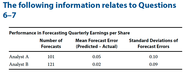
Problem 6
Investment analysts often use earnings per share (EPS) forecasts. One test of forecasting quality is the zero-mean test, which states that optimal forecasts should have a mean forecasting error of 0. (Forecasting error = Predicted value of variable − Actual value of variable.) You have collected data (shown in the table above) for two analysts who cover two different industries: Analyst A covers the telecom industry; Analyst B covers automotive parts and suppliers.
- A With μ as the population mean forecasting error, formulate null and alternative hypotheses for a zero-mean test of forecasting quality.
- B For Analyst A, using both a t-test and a z-test, determine whether to reject the null at the 0.05 and 0.01 levels of significance.
- C For Analyst B, using both a t-test and a z-test, determine whether to reject the null at the 0.05 and 0.01 levels of significance
Answer A
Null hypothesis is mean = 0
Alternative hypothesis is mean not equal to 0
Answer B
size <- 101

# mean
m <- 0.05

# sd
s <- 0.1
se <- s / sqrt(size)

# Levels for 0.05 significance

# alpha 0.05
a_5 <- 0.05

upper_5 <- qt(a_5/2, df = size - 1, lower.tail = F)
lower_5 <- qt(a_5/2, df = size - 1)

cat("At 0.05 significance level the upper and lover levels are", upper_5, 'and', lower_5)
## At 0.05 significance level the upper and lover levels are 1.983972 and -1.983972cat("\n")# Levels for 0.01 significance
# alpha 0.05
a_1 <- 0.01
upper_1 <- qt(a_1/2, df = size - 1, lower.tail = F)
lower_1 <- qt(a_1/2, df = size - 1)
cat("At 0.01 significance level the upper and lover levels are", upper_1, 'and', lower_1)## At 0.01 significance level the upper and lover levels are 2.625891 and -2.625891cat("\n")# Test at 0.05 signi
t <- (m - 0) / se
cat("The test statistic is", t)## The test statistic is 5.024938Since the test statistic is greater than 5.02, we can reject the null hypothesis at both 0.05 and 0.01 level.
Answer C
size <- 121

# mean
m <- 0.02

# sd
s <- 0.09
se <- s / sqrt(size)

# Levels for 0.05 significance

# alpha 0.05
a_5 <- 0.05

upper_5 <- qt(a_5/2, df = size - 1, lower.tail = F)
lower_5 <- qt(a_5/2, df = size - 1)

cat("At 0.05 significance level the upper and lover levels are", upper_5, 'and', lower_5)
## At 0.05 significance level the upper and lover levels are 1.97993 and -1.97993cat("\n")# Levels for 0.01 significance
# alpha 0.05
a_1 <- 0.01
upper_1 <- qt(a_1/2, df = size - 1, lower.tail = F)
lower_1 <- qt(a_1/2, df = size - 1)
cat("At 0.01 significance level the upper and lover levels are", upper_1, 'and', lower_1)## At 0.01 significance level the upper and lover levels are 2.617421 and -2.617421cat("\n")# Test at 0.05 signi
t <- (m - 0) / se
cat("The test statistic is", t)## The test statistic is 2.444444Since the test statistic is 2.44, we can reject the null hypothesis at 0.05 level. But 2.44 is less than 2.61, hence we cannot reject the null hypothesis at the 0.01 level of significance.
Problem 7
Reviewing the EPS forecasting performance data for Analysts A and B, you want to investigate whether the larger average forecast errors of Analyst A are due to chance or to a higher underlying mean value for Analyst A. Assume that the forecast errors of both analysts are normally distributed and that the samples are independent.
- A Formulate null and alternative hypotheses consistent with determining whether the population mean value of Analyst A’s forecast errors (μ1) are larger than Analyst B’s (μ2).
- B Identify the test statistic for conducting a test of the null hypothesis formulated in Part A.
- C Identify the rejection point or points for the hypothesis tested in Part A, at the 0.05 level of significance.
- D Determine whether or not to reject the null hypothesis at the 0.05 level of significance.
Answer A
μ1 = the population mean value of Analyst A’s forecast errors
μ2 = the population mean value of Analyst B’s forecast errors
Null Hypothesis μ1 - μ2 <= 0
Alternative Hypothesis μ1 - μ2 > 0
Answer B
Appropriate test is t-statistics using a pooled estimate of common variance and (101 + 121 - 2) = 220 degrees of freedom.
Answer C
# alpha
a <- 0.05

df = 220

t <- qt(a, df = df, lower.tail = F)
cat("We will reject the null hypothesis if the value is above", t)
## We will reject the null hypothesis if the value is above 1.651809Answer D
Using the formula for pooled variance
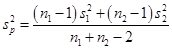
We find out the pooled estimate of variance
# pooled variance
v <- (((101 - 1) * (0.1) ^ 2) + ((121 - 1) * (0.09) ^ 2)) / (101 + 121 - 2)
v
## [1] 0.008963636The t test is
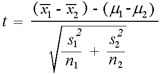
a <- 0.05
df <- 220

t_1 <- qt(a, df = df, lower.tail = F)

t <- ((0.05 - 0.02) - 0) / ((v / 101 + v / 121) ^ (1/2))

if (t > t_1) {
  cat("We reject the null hypothesis since test statistic", t," is greater than", t_1)
} else {

  cat("We do not reject the null hypothesis since test statistic", t,"is not greater than", t_1)
}
## We reject the null hypothesis since test statistic 2.351018 is greater than 1.651809Problem 8
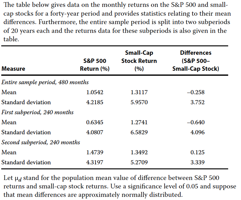
- A Formulate null and alternative hypotheses consistent with testing whether any difference exists between the mean returns on the S&P 500 and small-cap stocks.
- B Determine whether or not to reject the null hypothesis at the 0.05 significance level for the entire sample period.
- C Determine whether or not to reject the null hypothesis at the 0.05 significance level for the first subperiod.
- D Determine whether or not to reject the null hypothesis at the 0.05 significance level for the second subperiod.
Answer A
Let μd stand for the population mean value of difference between S&P 500 returns and small-cap stock returns.
Null hypothesis is μd = 0
Alternative hypothesis is μd != 0
Answer B
# alpha
a <- 0.05
n <- 480
df <- n - 1

upper <- qt(a/2, df = df, lower.tail = F)
lower <- qt(a/2, df = df, lower.tail = T)

cat("We will reject the null hypothesis if the test value is greater than", upper, "or less than", lower, "\n")
## We will reject the null hypothesis if the test value is greater than 1.964929 or less than -1.964929# mean difference
m <- -0.258
s <- 3.752
t <- (m - 0) / (s / sqrt(n))
if (t > upper) {
cat("We reject the null hypothesis since test statistic", t," is greater than", upper)
} else if (t < lower) {
cat("We reject the null hypothesis since test statistic", t," is less than", lower)
} else {
cat("We do not reject the null hypothesis since test statistic", t,"is not greater than", upper, "or less than", lower)
}## We do not reject the null hypothesis since test statistic -1.506529 is not greater than 1.964929 or less than -1.964929At 0.05 significan level we do not reject the null hypothesis.
Answer C
# alpha
a <- 0.05

# first sub period
n <- 240
df <- n - 1

upper <- qt(a/2, df = df, lower.tail = F)
lower <- qt(a/2, df = df, lower.tail = T)

cat("We will reject the null hypothesis if the test value is greater than", upper, "or less than", lower, "\n")
## We will reject the null hypothesis if the test value is greater than 1.969939 or less than -1.969939# mean difference
m <- -0.640
s <- 4.096
t <- (m - 0) / (s / sqrt(n))
if (t > upper) {
cat("We reject the null hypothesis since test statistic", t," is greater than", upper)
} else if (t < lower) {
cat("We reject the null hypothesis since test statistic", t," is less than", lower)
} else {
cat("We do not reject the null hypothesis since test statistic", t,"is not greater than", upper, "or less than", lower)
}## We reject the null hypothesis since test statistic -2.420615 is less than -1.969939At a 0.05 level of significance, we reject the null hypothesis. During this period small cap stocks significantly outperformed S&P 500 stocks.
Answer D
# alpha
a <- 0.05

# secod sub period
n <- 240
df <- n - 1

upper <- qt(a/2, df = df, lower.tail = F)
lower <- qt(a/2, df = df, lower.tail = T)

cat("We will reject the null hypothesis if the test value is greater than", upper, "or less than", lower, "\n")
## We will reject the null hypothesis if the test value is greater than 1.969939 or less than -1.969939# mean difference
m <- 0.125
s <- 3.339
t <- (m - 0) / (s / sqrt(n))
if (t > upper) {
cat("We reject the null hypothesis since test statistic", t," is greater than", upper)
} else if (t < lower) {
cat("We reject the null hypothesis since test statistic", t," is less than", lower)
} else {
cat("We do not reject the null hypothesis since test statistic", t,"is not greater than", upper, "or less than", lower)
}## We do not reject the null hypothesis since test statistic 0.5799616 is not greater than 1.969939 or less than -1.969939At 0.05 significan level, we do not reject the null hypothesis.
Problem 9
During a 10-year period, the standard deviation of annual returns on a portfolio you are analyzing was 15 percent a year. You want to see whether this record is sufficient evidence to support the conclusion that the portfolio’s underlying variance of return was less than 400, the return variance of the portfolio’s benchmark.
- A Formulate null and alternative hypotheses consistent with the verbal description of your objective.
- B Identify the test statistic for conducting a test of the hypotheses in Part A.
- C Identify the rejection point or points at the 0.05 significance level for the hypothesis tested in Part A.
- D Determine whether the null hypothesis is rejected or not rejected at the 0.05 level of significance.
Answer A
Null hypothesis is portfolio variance is greater than or equal to 400
Alternative hypothesis is portfolio variance is less than 400
Answer B
The test statistic is chi-square test with (10 - 1) = 9 degrees of freedom
Answer C
# alpha
a <- 0.05

df <- 10 - 1

level <- qchisq(a,df)

cat("We will reject the null hypothesis if test statistic is less than", level)
## We will reject the null hypothesis if test statistic is less than 3.325113Answer D
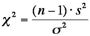
t <- ((10 - 1) * 15**2) / (400)

if (t < level) {

  cat("Reject the null hypothesis since", t, "is less than", level)

} else {

  cat("Do not reject the null hypothesis since", t, "is not less than", level)

}
## Do not reject the null hypothesis since 5.0625 is not less than 3.325113Problem 10
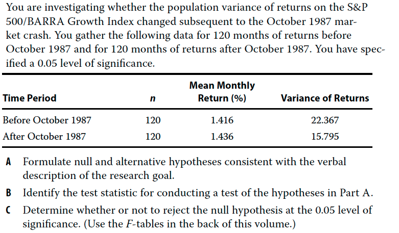
Answer A
We are investigating whether population variance of the index has changed subsequent to the October 1987 crash.
Null hypothesis is variance before is equal to variance after
Alternative hypothesis is variance before is not equal to variance afterwards
Answer B
To test the hypothesis, we use the F-test

Answer C
# alpha
a <- 0.05
df1 <- 119
df2 <- 119
critical_value <- qf(1 - a/2, df1 = df1, df2 = df2)

var_before <- 22.367
var_after <- 15.795

f_stat <- var_before / var_after

if (f_stat > critical_value) {

  cat("We reject the Null hypothesis, since", f_stat, "is greater than", critical_value)
} else {

  cat("We do not reject the Null hypothesis, since", f_stat, "is less than", critical_value)

}
## We do not reject the Null hypothesis, since 1.416081 is less than 1.434859Since 1.416081 is less than 1.434859, we do not reject the null hypothesis that the before and after variances are equal.
Problem 11
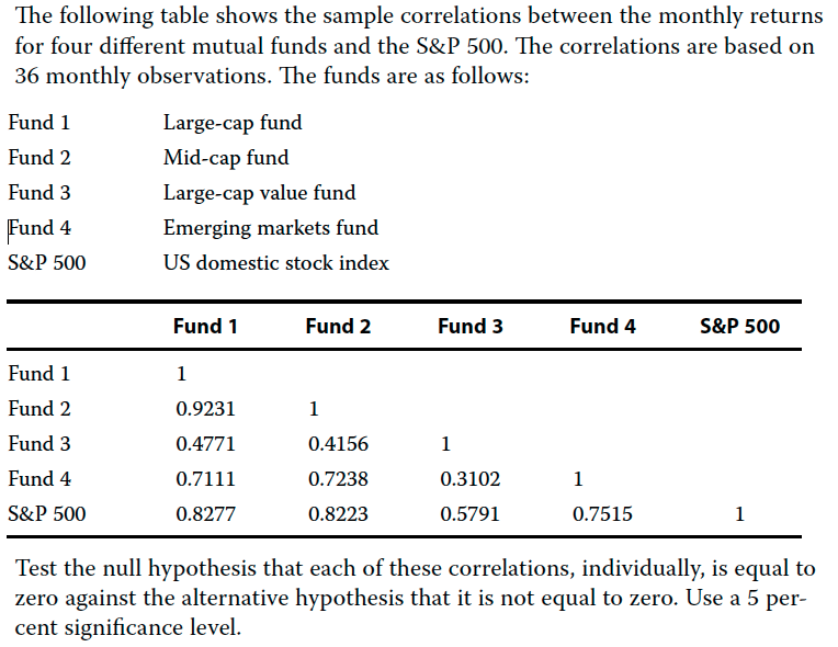
Instead of testing all the correlation, we will start with the smallest value. We will first test correlation between fund 3 and fund 4
We will use the following formula

# Correlation of fund 3 and 4
c_3_4 <- 0.3102

# t test
# alpha
a <- 0.05
df <- 36 - 2

critical_value <- qt(a/2, df = df, lower.tail = F)


t <- c_3_4 * sqrt(df - 2 / (1 - c_3_4))

if (t > critical_value) {

  cat("We reject the null hypothesis since", t, "is greater than", critical_value)

} else {

  cat("We do not reject the null hypothesis since", t, "is less than", critical_value)
}
## We do not reject the null hypothesis since 1.729921 is less than 2.032245We can now try the next smallest correlation. Its the correlation between Fund 3 and Fund 2.
# Correlation of fund 3 and 4
c_3_4 <- 0.4156

# t test
# alpha
a <- 0.05
df <- 36 - 2

critical_value <- qt(a/2, df = df, lower.tail = F)


t <- c_3_4 * sqrt(df - 2 / (1 - c_3_4))

if (t > critical_value) {

  cat("We reject the null hypothesis since", t, "is greater than", critical_value)

} else {

  cat("We do not reject the null hypothesis since", t, "is less than", critical_value)

}
## We reject the null hypothesis since 2.298147 is greater than 2.032245At a 0.05 level we can reject the null hypothesis. Since all other correlation are larger than this, we can assume they are all statistically significant.
Problem 12
In the step “stating a decision rule” in testing a hypothesis, which of the following elements must be specified?
- A Critical value
- B Power of a test
- C Value of a test statistic
A - Critical Value
Problem 13
Which of the following statements is correct with respect to the null hypothesis?
- A It is considered to be true unless the sample provides evidence showing it is false.
- B It can be stated as “not equal to” provided the alternative hypothesis is stated as “equal to.”
- C In a two-tailed test, it is rejected when evidence supports equality between the hypothesized value and population parameter.
A - It is considered to be true unless the sample provides evidence showing it is false.
Problem 14
An analyst is examining a large sample with an unknown population variance. To test the hypothesis that the historical average return on an index is less than or equal to 6%, which of the following is the most appropriate test?
- A One-tailed z-test
- B Two-tailed z-test
- C One-tailed F-test
A - One-tailed z-test
Problem 15
A hypothesis test for a normally-distributed population at a 0.05 significance level implies a:
- A 95% probability of rejecting a true null hypothesis.
- B 95% probability of a Type I error for a two-tailed test.
- C 5% critical value rejection region in a tail of the distribution for a one-tailed test.
C - 5% critical value rejection region in a tail of the distribution for a one-tailed test.
Problem 16
Which of the following statements regarding a one-tailed hypothesis test is correct?
- A The rejection region increases in size as the level of significance becomes smaller.
- B A one-tailed test more strongly reflects the beliefs of the researcher than a two-tailed test.
- C The absolute value of the rejection point is larger than that of a two-tailed test at the same level of significance.
B - A one-tailed test more strongly reflects the beliefs of the researcher than a two-tailed test.
Problem 17
The value of a test statistic is best described as the basis for deciding whether to:
- A reject the null hypothesis.
- B accept the null hypothesis.
- C reject the alternative hypothesis.
A - reject the null hypothesis.
Problem 18
Which of the following is a Type I error?
- A Rejecting a true null hypothesis
- B Rejecting a false null hypothesis
- C Failing to reject a false null hypothesis
A - Rejecting a true null hypothesis
Problem 19
A Type II error is best described as:
- A rejecting a true null hypothesis.
- B failing to reject a false null hypothesis.
- C failing to reject a false alternative hypothesis.
B - failing to reject a false null hypothesis.
Problem 20
The level of significance of a hypothesis test is best used to:
- A calculate the test statistic.
- B define the test’s rejection points.
- C specify the probability of a Type II error.
B - define the test’s rejection points.
Problem 22
All else equal, is specifying a smaller significance level in a hypothesis test likely to increase the probability of a:
tabl <- "  # Problem 22
 Type I Error  | Type II Error |
|---------------|:-------------:|
|A| No            | No            |
|B| No            | Yes           |
|C| Yes           | No            |
"

cat(tabl)
## # Problem 22
## Type I Error | Type II Error |
## |---------------|:-------------:|
## |A| No | No |
## |B| No | Yes |
## |C| Yes | No |B - Specifying a small significance level increases the chance of Type to error and not Type I error.
Problem 23
The probability of correctly rejecting the null hypothesis is the:
- A p-value.
- B power of a test.
- C level of significance.
B - power of a test
Problem 24
The power of a hypothesis test is:
- A equivalent to the level of significance.
- B the probability of not making a Type II error.
- C unchanged by increasing a small sample size.
B - the probability of not making a Type II error.
Problem 25
When making a decision in investments involving a statistically significant result, the:
- A economic result should be presumed meaningful.
- B statistical result should take priority over economic considerations.
- C economic logic for the future relevance of the result should be further explored.
C - economic logic for the future relevance of the result should be further explored.
Problem 26
An analyst tests the profitability of a trading strategy with the null hypothesis being that the average abnormal return before trading costs equals zero. The calculated t-statistic is 2.802, with critical values of ± 2.756 at significance level α = 0.01. After considering trading costs, the strategy’s return is near zero. The results are most likely:
- A statistically but not economically significant.
- B economically but not statistically significant.
- C neither statistically nor economically significant.
A - statistically but not economically significant.
Problem 27
Which of the following statements is correct with respect to the p-value?
- A It is a less precise measure of test evidence than rejection points.
- B It is the largest level of significance at which the null hypothesis is rejected.
- C It can be compared directly with the level of significance in reaching test conclusions.
C - It can be compared directly with the level of significance in reaching test conclusions.
Problem 28
Which of the following represents a correct statement about the p-value?
- A The p-value offers less precise information than does the rejection points approach.
- B A larger p-value provides stronger evidence in support of the alternative hypothesis.
- C A p-value less than the specified level of significance leads to rejection of the null hypothesis.
C - A p-value less than the specified level of significance leads to rejection of the null hypothesis.
Problem 29
Which of the following statements on p-value is correct?
- A The p-value is the smallest level of significance at which H0 can be rejected.
- B The p-value indicates the probability of making a Type II error.
- C The lower the p-value, the weaker the evidence for rejecting the H0.
A - The p-value is the smallest level of significance at which H0 can be rejected.
Problem 30
The following table shows the significance level (α) and the p-value for three hypothesis tests.
tabl <- "  # Problem 30 Table
| Test        | alpha| p-value|
|-------------|:----:|-------:|
| Test 1      | 0.05 | 0.10 |
| Test 2      | 0.10 | 0.08 |
| Test 3      | 0.10 | 0.05 |
"
cat(tabl)
## # Problem 30 Table
## | Test | alpha| p-value|
## |-------------|:----:|-------:|
## | Test 1 | 0.05 | 0.10 |
## | Test 2 | 0.10 | 0.08 |
## | Test 3 | 0.10 | 0.05 |The evidence for rejecting H0 is strongest for:
- A Test 1.
- B Test 2.
- C Test 3.
C - Test 3
Problem 31
Which of the following tests of a hypothesis concerning the population mean is most appropriate?
- A A z-test if the population variance is unknown and the sample is small
- B A z-test if the population is normally distributed with a known variance
- C A t-test if the population is non-normally distributed with unknown variance and a small sample
B - A z-test if the population is normally distributed with a known variance
Problem 32
For a small sample with unknown variance, which of the following tests of a hypothesis concerning the population mean is most appropriate?
- A A t-test if the population is normally distributed
- B A t-test if the population is non-normally distributed
- C A z-test regardless of the normality of the population distribution
A - A t-test if the population is normally distributed
Problem 33
For a small sample from a normally distributed population with unknown variance, the most appropriate test statistic for the mean is the:
- A z-statistic.
- B t-statistic.
- C χ2 statistic.
B - t-statistic.
Problem 34
An investment consultant conducts two independent random samples of 5-year performance data for US and European absolute return hedge funds. Noting a 50 basis point return advantage for US managers, the consultant decides to test whether the two means are statistically different from one another at a 0.05 level of significance. The two populations are assumed to be normally distributed with unknown but equal variances. Results of the hypothesis test are contained in the tables below.
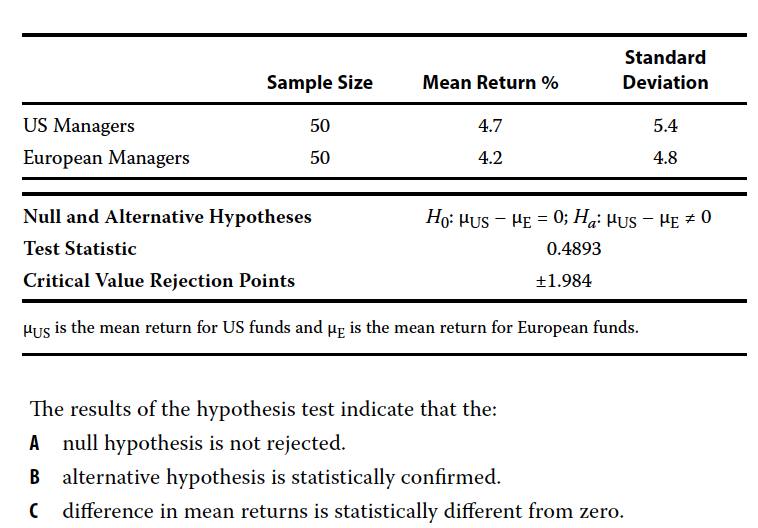
A - null hypothesis is not rejected.
Problem 35
A pooled estimator is used when testing a hypothesis concerning the:
- A equality of the variances of two normally distributed populations.
- B difference between the means of two at least approximately normally distributed populations with unknown but assumed equal variances.
- C difference between the means of two at least approximately normally distributed populations with unknown and assumed unequal variances.
B - difference between the means of two at least approximately normally distributed populations with unknown but assumed equal variances.
Problem 36
When evaluating mean differences between two dependent samples, the most appropriate test is a:
- A chi-square test.
- B paired comparisons test.
- C z-test.
B - paired comparisons test.
Problem 37
A fund manager reported a 2% mean quarterly return over the past ten years for its entire base of 250 client accounts that all follow the same investment strategy. A consultant employing the manager for 45 client accounts notes that their mean quarterly returns were 0.25% less over the same period. The consultant tests the hypothesis that the return disparity between the returns of his clients and the reported returns of the fund manager’s 250 client accounts are significantly different from zero. Assuming normally distributed populations with unknown population variances, the most appropriate test statistic is:
- A a paired comparisons t-test.
- B a t-test of the difference between the two population means.
- C an approximate t-test of mean differences between the two populations.
A - a paired comparisons t-test.
Problem 38
A chi-square test is most appropriate for tests concerning:
- A a single variance.
- B differences between two population means with variances assumed to be equal.
- C differences between two population means with variances assumed to not be equal.
A - a single variance.
Problem 39
Which of the following should be used to test the difference between the variances of two normally distributed populations?
- A t-test
- B F-test
- C Paired comparisons test
B - F-test
Problem 40
Jill Batten is analyzing how the returns on the stock of Stellar Energy Corp. are related with the previous month’s percent change in the US Consumer Price Index for Energy (CPIENG). Based on 248 observations, she has computed the sample correlation between the Stellar and CPIENG variables to be −0.1452. She also wants to determine whether the sample correlation is statistically significant. The critical value for the test statistic at the 0.05 level of significance is approximately 1.96. Batten should conclude that the statistical relationship between Stellar and CPIENG is:
- A significant, because the calculated test statistic has a lower absolute value than the critical value for the test statistic.
- B significant, because the calculated test statistic has a higher absolute value than the critical value for the test statistic.
- C not significant, because the calculated test statistic has a higher absolute value than the critical value for the test statistic.
# Correlation
r <- -0.1452

n <- 248

# Test staistic
t <- r * sqrt((n - 2) / (1 - r**2))


# Critical value is
critical_value <- 1.96

if (abs(critical_value) > t) {

  cat("The correlation coefficient is statistically significant since", abs(t), "greater than", critical_value)
}
## The correlation coefficient is statistically significant since 2.301766 greater than 1.96B - significant, because the calculated test statistic has a higher absolute value than the critical value for the test statistic.
Problem 41
In which of the following situations would a non-parametric test of a hypothesis most likely be used?
- A The sample data are ranked according to magnitude.
- B The sample data come from a normally distributed population.
- C The test validity depends on many assumptions about the nature of the population.
A - The sample data are ranked according to magnitude.
Problem 42
An analyst is examining the monthly returns for two funds over one year. Both funds’ returns are non-normally distributed. To test whether the mean return of one fund is greater than the mean return of the other fund, the analyst can use:
- A a parametric test only.
- B a nonparametric test only.
- C both parametric and nonparametric tests.
B - a nonparametric test only.