Quantitative Investment Analysis - Chapter 8
library(tidyverse)
library(knitr)
library(kableExtra)
In this post we will solve the end of the chapter practice problems from chapter 7 of the book.
Problem 1
Julie Moon is an energy analyst examining electricity, oil, and natural gas consumption in different regions over different seasons. She ran a regression explaining the variation in energy consumption as a function of temperature. The total variation of the dependent variable was 140.58, the explained variation was 60.16, and the unexplained variation was 80.42. She had 60 monthly observations.
- A Compute the coefficient of determination.
- B What was the sample correlation between energy consumption and temperature?
- C Compute the standard error of the estimate of Moon’s regression model.
- D Compute the sample standard deviation of monthly energy consumption.
# total variation
t_v <- 140.58

# explained variation
e_v <- 60.16

# unexplained variation
ue_v <- 80.42

# Coef of determination
coef_d <- e_v / t_v

cat("The coefficient of determination is", coef_d)
## The coefficient of determination is 0.4279414A - The coefficient of determination is 0.4279414
corr <- sqrt(coef_d)
cat("The sample correlation between energy consumption and temperature is", corr)
## The sample correlation between energy consumption and temperature is 0.6541723B - The sample correlation between energy consumption and temperature is 0.6541723
# The standard error of the estimate is the square root of the
# coefficient of non-determination divided by it's degrees of freedom

# number of observations
n <- 60

# se
se <- sqrt(ue_v / (n - 2))

cat("The standard error of the estimate of Moon’s regression model is", se)
## The standard error of the estimate of Moon’s regression model is 1.177519C- The standard error of the estimate of Moon’s regression model is 1.177519
# The sample variance of the dependent variable is

sv <- t_v / (n - 1)

# sample standard deviation is

s <- sqrt(sv)

cat("The sample standard deviation of monthly energy consumption is", s)
## The sample standard deviation of monthly energy consumption is 1.543604D - The sample standard deviation of monthly energy consumption is 1.543604
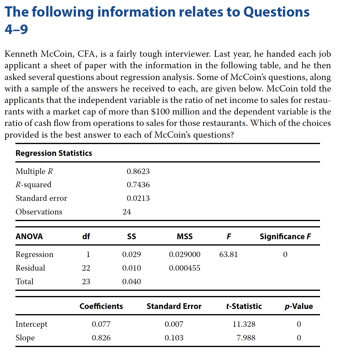
Problem 4
What is the value of the coefficient of determination?
- A 0.8261.
- B 0.7436.
- C 0.8623.
B - 0.7436
Problem 5
Suppose that you deleted several of the observations that had small residual values. If you re-estimated the regression equation using this reduced sample, what would likely happen to the standard error of the estimate and the R-squared?
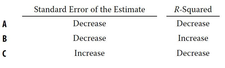
C - Deleting observations with small residual values will increase standard error and decrease R-Squared
Problem 6
What is the correlation between X and Y?
- A −0.7436.
- B 0.7436.
- C 0.8623.
# Coef of Determination aka R-squared
coef_d <- 0.7436

corr <- sqrt(coef_d)
corr
## [1] 0.8623224C - 0.8623
Problem 7
Where did the F-value in the ANOVA table come from?
- A You look up the F-value in a table. The F depends on the numerator and denominator degrees of freedom.
- B Divide the “Mean Square” for the regression by the “Mean Square” of the residuals.
- C The F-value is equal to the reciprocal of the t-value for the slope coefficient.
B - Divide the “Mean Square” for the regression by the “Mean Square” of the residuals.
Problem 8
If the ratio of net income to sales for a restaurant is 5 percent, what is the predicted ratio of cash flow from operations to sales?
- A 0.007 + 0.103(5.0) = 0.524.
- B 0.077 − 0.826(5.0) = −4.054.
- C 0.077 + 0.826(5.0) = 4.207.
C - 0.077 + 0.826(5.0) = 4.207.
Problem 9
Is the relationship between the ratio of cash flow to operations and the ratio of net income to sales significant at the 5 percent level?
- A No, because the R-squared is greater than 0.05.
- B No, because the p-values of the intercept and slope are less than 0.05.
- C Yes, because the p-values for F and t for the slope coefficient are less than 0.05.
C - Yes, because the p-values for F and t for the slope coefficient are less than 0.05.
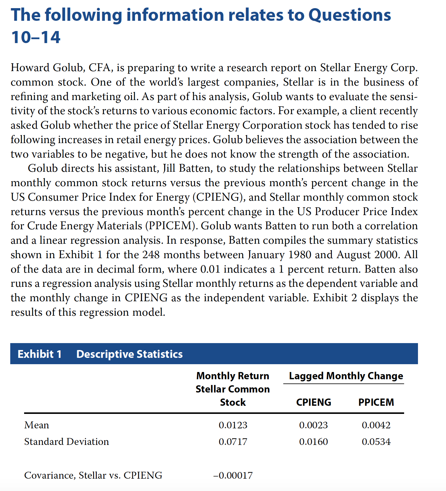
Problem 10
Did Batten’s regression analyze cross-sectional or time-series data, and what was the expected value of the error term from that regression?
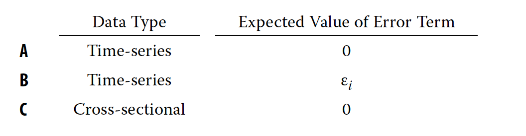
A - The data are time-series and the expected value of the error term is 0
Problem 11
Based on the regression, which used data in decimal form, if the CPIENG decreases by 1.0 percent, what is the expected return on Stellar common stock during the next period?
- A 0.0073 (0.73 percent).
- B 0.0138 (1.38 percent).
- C 0.0203 (2.03 percent).
# beta
b <- -0.6486
# alpha
a <- 0.0138

exp_ret <- a + b * (-0.01)
exp_ret
## [1] 0.020286C - 0.0203
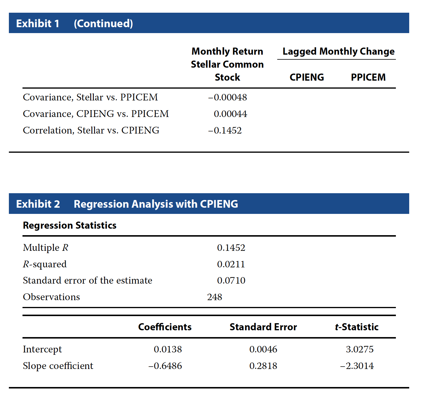
Problem 12
Based on Batten’s regression model, the coefficient of determination indicates that:
- A Stellar’s returns explain 2.11 percent of the variability in CPIENG.
- B Stellar’s returns explain 14.52 percent of the variability in CPIENG.
- C Changes in CPIENG explain 2.11 percent of the variability in Stellar’s returns.
C - Changes in CPIENG explain 2.11 percent of the variability in Stellar’s returns.
Problem 13
For Batten’s regression model, the standard error of the estimate shows that the standard deviation of:
- A the residuals from the regression is 0.0710.
- B values estimated from the regression is 0.0710.
- C Stellar’s observed common stock returns is 0.0710.
A - The residuals from the regression is 0.0710.
Problem 14
For the analysis run by Batten, which of the following is an incorrect conclusion from the regression output?
- A The estimated intercept coefficient from Batten’s regression is statistically significant at the 0.05 level.
- B In the month after the CPIENG declines, Stellar’s common stock is expected to exhibit a positive return.
- C Viewed in combination, the slope and intercept coefficients from Batten’s regression are not statistically significant at the 0.05 level
C - Viewed in combination, the slope and intercept coefficients from Batten’s regression are not statistically significant at the 0.05 level
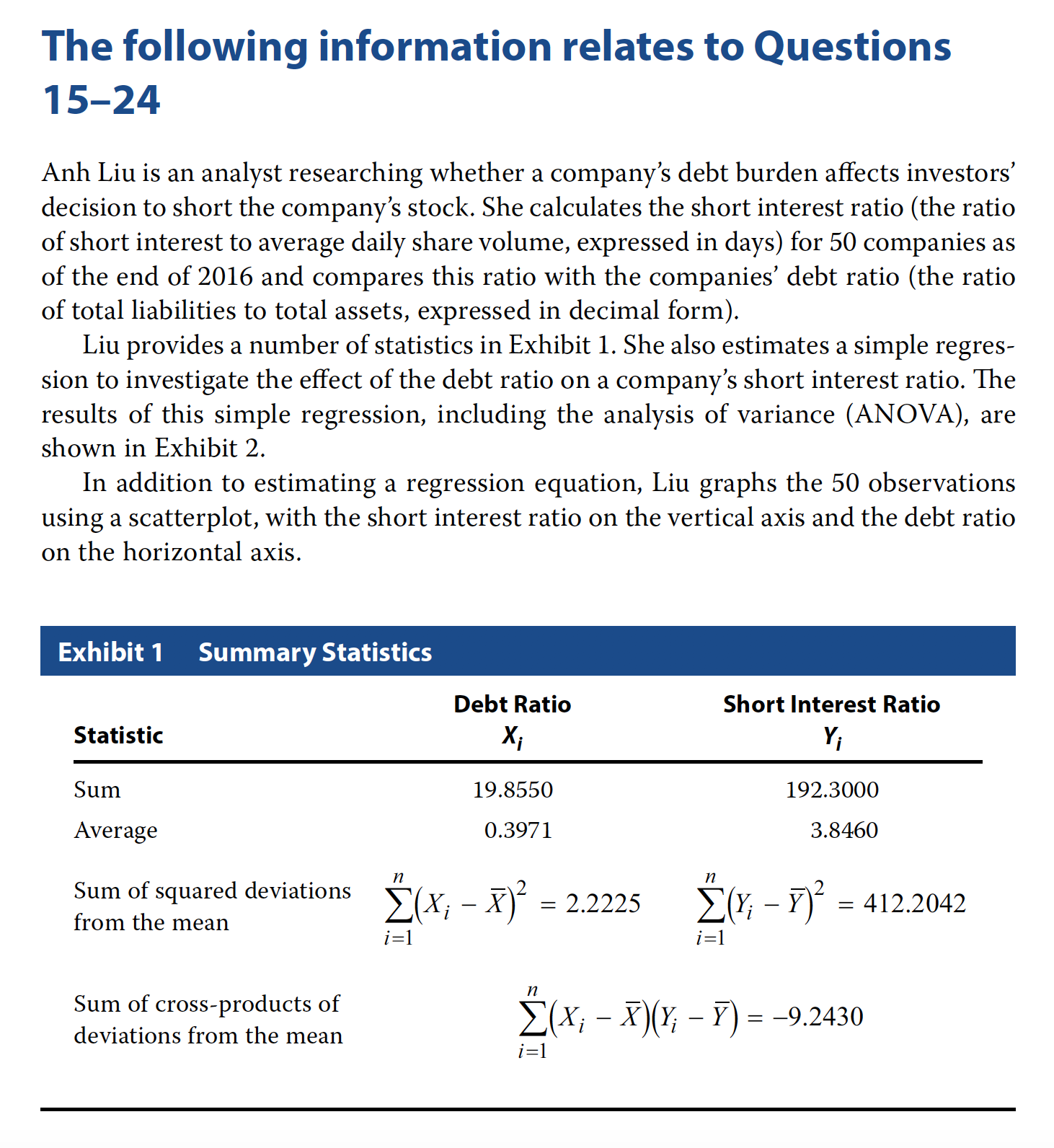
Problem 15
Based on Exhibits 1 and 2, if Liu were to graph the 50 observations, the scatterplot summarizing this relation would be best described as:
- A horizontal.
- B upward sloping.
- C downward sloping.
C - downward sloping.
Problem 16
Based on Exhibit 1, the sample covariance is closest to:
- A −9.2430.
- B −0.1886.
- C 8.4123.
# Its sum of cross product
# of deviations from the mean
# divided by n - 1

sum_cp <- -9.2430

n <- 50

sum_cp / (n - 1)
## [1] -0.1886327B - -0.1886327
Problem 17
Based on Exhibit 1, the correlation between the debt ratio and the short interest ratio is closest to:
- A −0.3054.
- B 0.0933.
- C 0.3054.
# R-squared

r2 <- 0.0933

# corr

corr <- sqrt(r2)

# Since the coefficient sign is negative
# our correlation is also negative

-corr
## [1] -0.3054505A - -0.3054
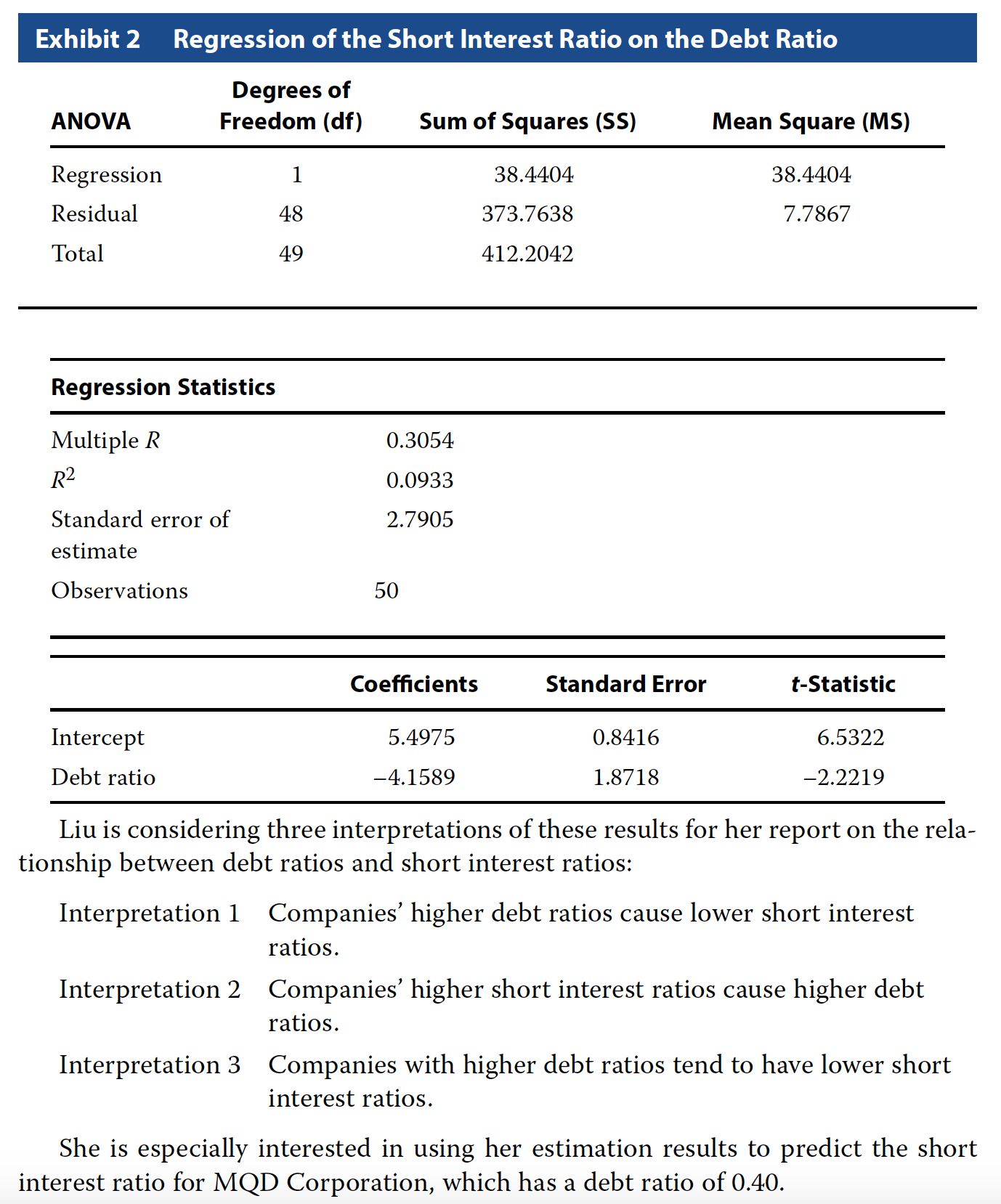
Problem 18
Which of the interpretations best describes Liu’s findings for her report?
- A Interpretation 1
- B Interpretation 2
- C Interpretation 3
C - Interpretation 3
Problem 19
The dependent variable in Liu’s regression analysis is the:
- A intercept.
- B debt ratio.
- C short interest ratio.
C - short interest ratio.
Problem 20
Based on Exhibit 2, the degrees of freedom for the t-test of the slope coefficient in this regression are:
- A 48.
- B 49.
- C 50.
A - 48
Problem 21
The upper bound for the 95% confidence interval for the coefficient on the debt ratio in the regression is closest to:
- A −1.0199.
- B −0.3947.
- C 1.4528.
# Critical value at 95% level
# Two tail

# alpha
a <- 0.05

# critical level
critical <- qt(a / 2, df = 48, lower.tail = F)

upper <- -4.1589 + (critical * 1.8717)

upper
## [1] -0.3955949B - -0.395
Problem 22
Which of the following should Liu conclude from these results shown in Exhibit 2?
- A The average short interest ratio is 5.4975.
- B The estimated slope coefficient is statistically significant at the 0.05 level.
- C The debt ratio explains 30.54% of the variation in the short interest ratio.
B - The estimated slope coefficient is statistically significant at the 0.05 level.
Problem 23
Based on Exhibit 2, the short interest ratio expected for MQD Corporation is closest to:
- A 3.8339.
- B 5.4975.
- C 6.2462.
5.4975 + (-4.1589 * 0.4)## [1] 3.83394A - 3.8339
Problem 24
Based on Liu’s regression results in Exhibit 2, the F-statistic for testing whether the slope coefficient is equal to zero is closest to:
- A −2.2219.
- B 3.5036.
- C 4.9367.
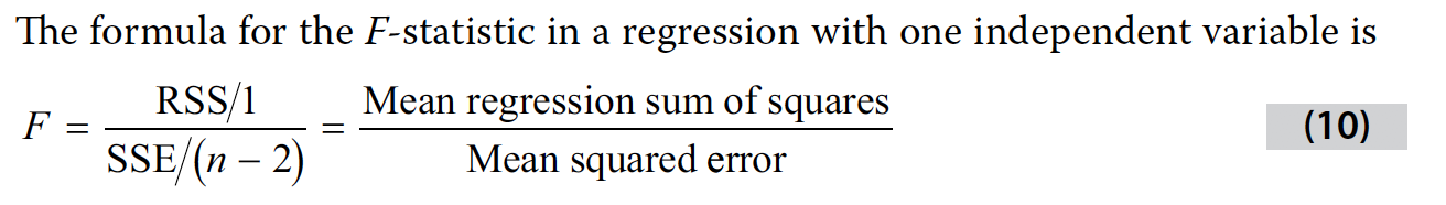
F = 38.4404 / 7.7867
F
## [1] 4.936674C - 4.9367
Problem 25
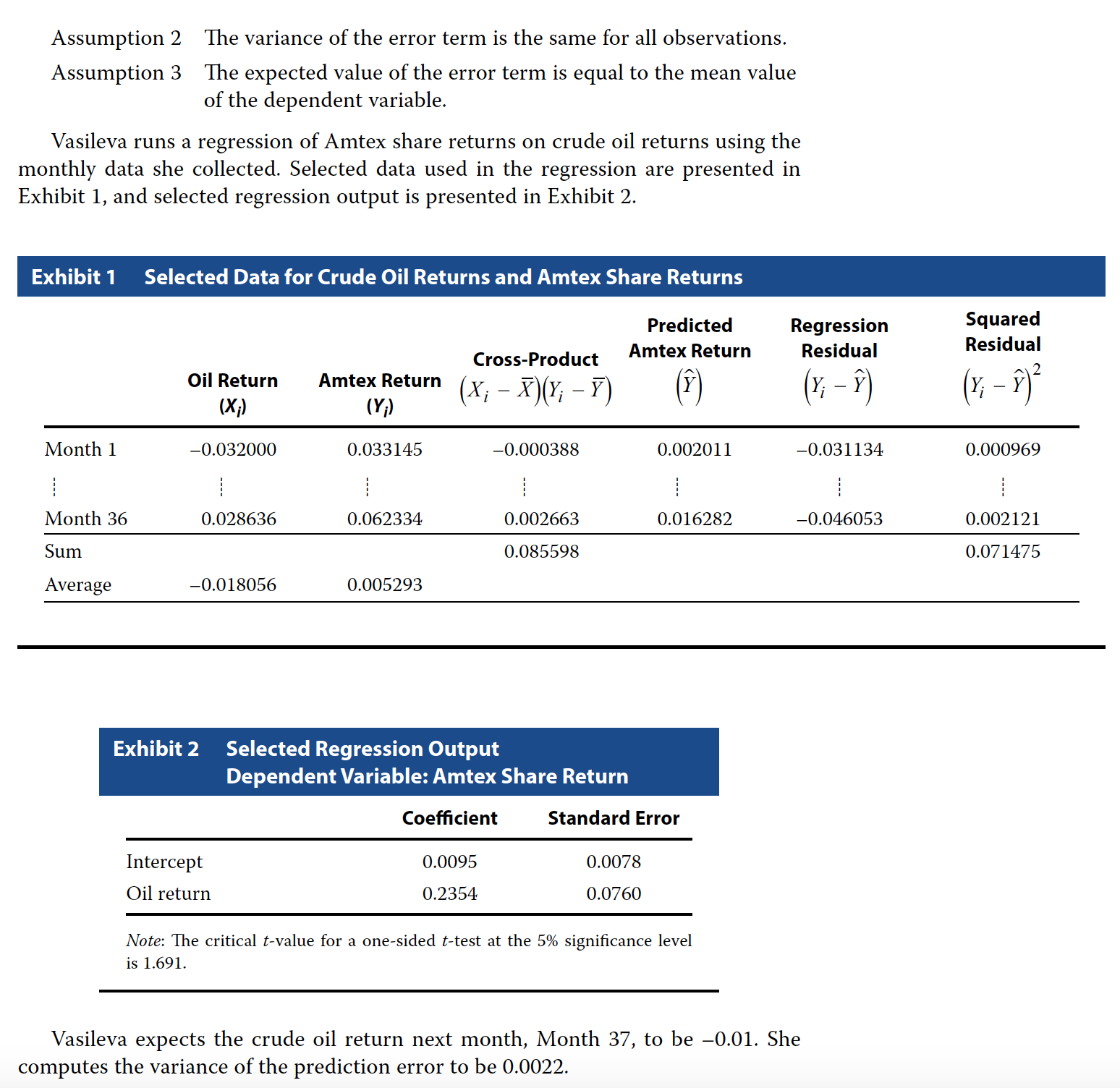
Which of Vasileva’s assumptions regarding regression analysis is incorrect?
- A Assumption 1
- B Assumption 2
- C Assumption 3
C - Assumption 3
Problem 26
Based on Exhibit 1, the standard error of the estimate is closest to:
- A 0.044558.
- B 0.045850.
- C 0.050176.
# from the table
# sum of squared residual

ssr <- 0.071475

# observations 36
n = 36
sse <- sqrt(ssr/(n - 2))

sse
## [1] 0.04584982B - 0.045850
Problem 27
Based on Exhibit 2, Vasileva should reject the null hypothesis that:
- A the slope is less than or equal to 0.15.
- B the intercept is less than or equal to 0.
- C crude oil returns do not explain Amtex share returns.
C - crude oil returns do not explain Amtex share returns.
Problem 28
Based on Exhibit 2, Vasileva should compute the:
- A coefficient of determination to be 0.4689.
- B 95% confidence interval for the intercept to be –0.0037 to 0.0227.
- C 95% confidence interval for the slope coefficient to be 0.0810 to 0.3898.
# alpha 0.05

a <- 0.05
df <- 36 -2

critical <- qt(a / 2,df = df, lower.tail = F)

upper  <- 0.2354 + (critical * 0.076)
lower  <- 0.2354 - (critical * 0.076)

cat("Range is", lower, "and", upper)
## Range is 0.3898506 and 0.08094942C - 95% confidence interval for the slope coefficient to be 0.0810 to 0.3898.
Problem 29
Based on Exhibit 2 and Vasileva’s prediction of the crude oil return for month 37, the estimate of Amtex share return for month 37 is closest to:
- A –0.0024.
- B 0.0071.
- C 0.0119.
0.0095 + (0.2354 * -0.01)## [1] 0.007146B - 0.0071.
Problem 30
Using information from Exhibit 2, Vasileva should compute the 95% prediction interval for Amtex share return for month 37 to be:
- A –0.0882 to 0.1025.
- B –0.0835 to 0.1072.
- C 0.0027 to 0.0116.
# variance
v <- 0.0022
# sd
s <- sqrt(v)

# predicted value

p <- 0.0095 + (0.2354 * -0.01)

# We know the critical value from above

# Lower limit for prediction
lower <- p - (critical * s)
upper <- p + (critical * s)

cat("Prediction range is", lower, "and", upper)
## Prediction range is 0.1024667 and -0.08817472A –0.0882 to 0.1025.
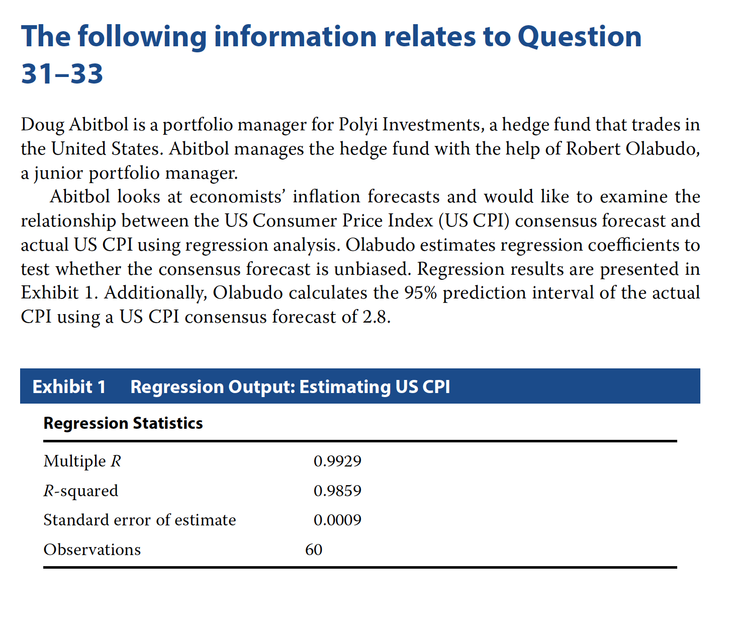
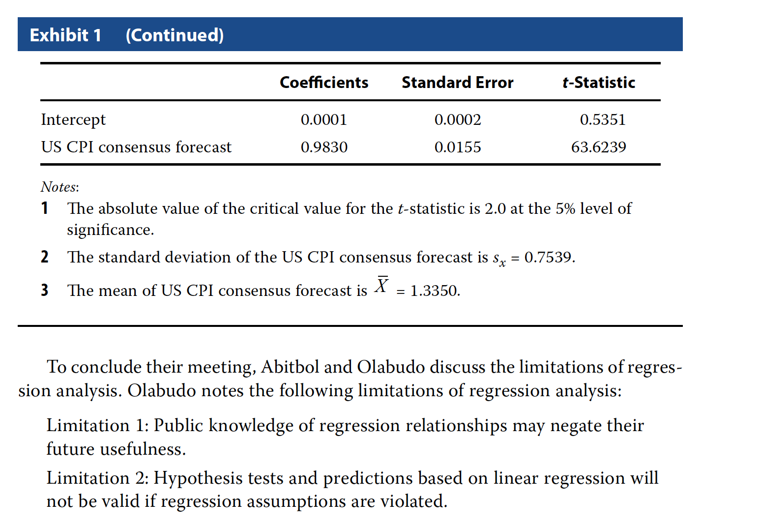
Problem 31
Based on Exhibit 1, Olabudo should:
- A conclude that the inflation predictions are unbiased.
- B reject the null hypothesis that the slope coefficient equals 1.
- C reject the null hypothesis that the intercept coefficient equals 0.
A - conclude that the inflation predictions are unbiased.
Problem 33
Which of Olabudo’s noted limitations of regression analysis is correct? A Only Limitation 1 B Only Limitation 2 C Both Limitation 1 and Limitation 2
C - Both Limitation 1 and Limitation 2