How to calculate portfolio returns in Python
Calculating portfolio returns in Python
In this post we will learn to calculate the portfolio returns in Python. Since we are not aware of any modules that perform such calculations we will perform this calculation manually.
Calculating portfolio returns using the formula
A portfolio return is the weighted average of individual assets in the portfolio.
Here is what we need
- Asset symbols that make up our portfolio
- Price data for the assets
- weights of assets
- Calculating the weighted average of our assets returns
- Adding them to get the portfolio returns
Lets first load the modules
import pandas as pd
import numpy as np
import matplotlib.pyplot as plt
import pandas_datareader as web
We will invest in the following assets
- Aggregate Bonds ETF (BND) 10%
- Small Cap ETF (VB) 20%
- Developed markets ETF (VEA) 25%
- S&P 500 ETF (VOO) 25%
- Emerging Markets ETF (VWO) 20%
So lets assign our assets to the symbols variable.
symbols = ['VOO','VEA', 'VB', 'VWO','BND']Next we download the price data for the assets.
price_data = web.get_data_yahoo(symbols,
                               start = '2013-01-01',
                               end = '2018-03-01')
Now that we have the price data lets look at the head of this data.
print(price_data.head())## Attributes High ... Adj Close
## Symbols BND VB ... VOO VWO
## Date ...
## 2013-01-02 83.940002 83.209999 ... 117.851250 38.347870
## 2013-01-03 83.930000 83.690002 ... 117.745369 38.120152
## 2013-01-04 83.779999 83.919998 ... 118.239380 38.187622
## 2013-01-07 83.760002 83.639999 ... 117.921799 37.858707
## 2013-01-08 83.849998 83.610001 ... 117.568985 37.546669
##
## [5 rows x 30 columns]But we just need the Adjusted Closing price for our returns calculations. So lets select that columns.
price_data = price_data['Adj Close']
print(price_data.head())
## Symbols BND VB VEA VOO VWO
## Date
## 2013-01-02 71.491119 75.985794 29.420095 117.851250 38.347870
## 2013-01-03 71.278122 75.940125 29.124334 117.745369 38.120152
## 2013-01-04 71.388893 76.515572 29.288649 118.239380 38.187622
## 2013-01-07 71.337738 76.287193 29.140768 117.921799 37.858707
## 2013-01-08 71.405899 76.141068 28.984674 117.568985 37.546669We can see that pandas has sorted our columns alphabetically so we need to align our weights correctly to the column names.
w = [0.1,0.2,0.25,0.25,0.2]A quick check to see if our weights add to one.
print(sum(w))## 1.0Now we will calculate the asset returns in our portfolio.
ret_data = price_data.pct_change()[1:]
print(ret_data.head())
## Symbols BND VB VEA VOO VWO
## Date
## 2013-01-03 -0.002979 -0.000601 -0.010053 -0.000898 -0.005938
## 2013-01-04 0.001554 0.007578 0.005642 0.004196 0.001770
## 2013-01-07 -0.000717 -0.002985 -0.005049 -0.002686 -0.008613
## 2013-01-08 0.000955 -0.001915 -0.005357 -0.002992 -0.008242
## 2013-01-09 -0.000358 0.004319 0.004818 0.003001 0.005840Next we can calculate the weighted returns of our assets.
weighted_returns = (w * ret_data)
print(weighted_returns.head())
## Symbols BND VB VEA VOO VWO
## Date
## 2013-01-03 -0.000298 -0.000120 -0.002513 -0.000225 -0.001188
## 2013-01-04 0.000155 0.001516 0.001410 0.001049 0.000354
## 2013-01-07 -0.000072 -0.000597 -0.001262 -0.000671 -0.001723
## 2013-01-08 0.000096 -0.000383 -0.001339 -0.000748 -0.001648
## 2013-01-09 -0.000036 0.000864 0.001205 0.000750 0.001168Next the portfolio returns are simply the sum of the weighted returns of the assets. So lets add the rows.
port_ret = weighted_returns.sum(axis=1)
# axis =1 tells pandas we want to add
# the rows
Lets plot the histogram of the returns.
fig = plt.figure()
ax1 = fig.add_axes([0.1,0.1,0.8,0.8])
ax1.hist(port_ret, bins = 60)
ax1.set_xlabel('Portfolio returns')
ax1.set_ylabel("Freq")
ax1.set_title("Portfolio Returns calculated manually")
plt.show(); 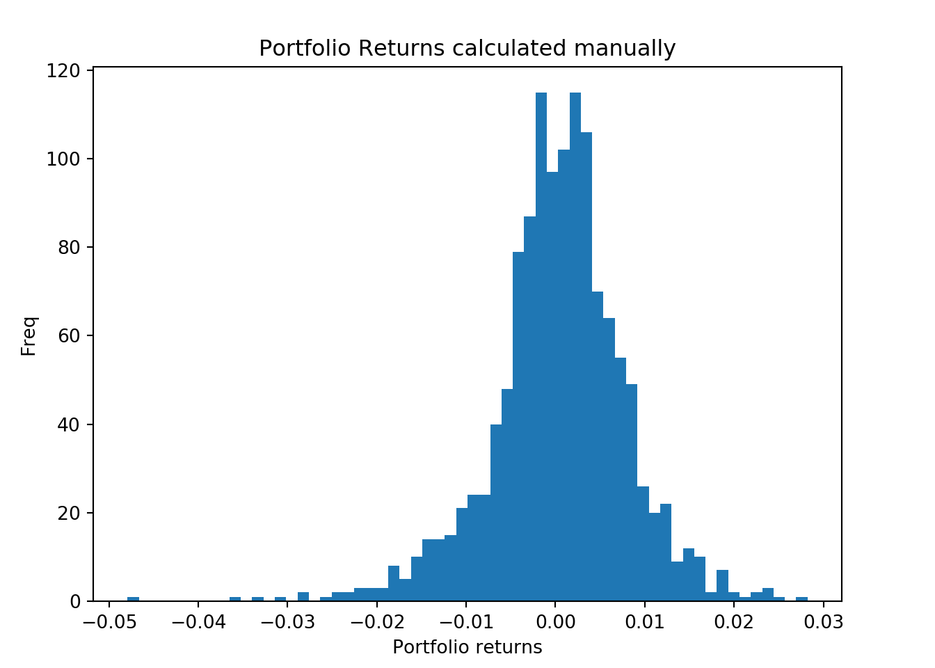
Tidy method in Python
In the example given in the R post we calculated the portfolio returns using the tidy dataframe. We can also calculate the returns using a tidy method in Python. To do that we need to reshape our returns dataframe and create a new weights table. We will then join the two and calculate the portfolio returns.
First lets create a weights table.
wts_table = pd.DataFrame({'symbol':symbols,
                          'wts':[0.25,0.25,0.2,0.2,0.1]})
print(wts_table.head())
## symbol wts
## 0 VOO 0.25
## 1 VEA 0.25
## 2 VB 0.20
## 3 VWO 0.20
## 4 BND 0.10Next we will transform our returns data into a tidy data. First we need to reset the index and make the Date index into a separate column.
ret_data_tidy = pd.melt(ret_data.reset_index(),
        id_vars='Date',
        var_name='symbol',
        value_name='ret')

print(ret_data_tidy.head())
## Date symbol ret
## 0 2013-01-03 BND -0.002979
## 1 2013-01-04 BND 0.001554
## 2 2013-01-07 BND -0.000717
## 3 2013-01-08 BND 0.000955
## 4 2013-01-09 BND -0.000358We can see that the assets have been stacked on top of one another and Date has a separate column. Next we can merge our data by symbols.
ret_data_tidy_wts = pd.merge(ret_data_tidy,wts_table,on="symbol")
print(ret_data_tidy_wts.head())
## Date symbol ret wts
## 0 2013-01-03 BND -0.002979 0.1
## 1 2013-01-04 BND 0.001554 0.1
## 2 2013-01-07 BND -0.000717 0.1
## 3 2013-01-08 BND 0.000955 0.1
## 4 2013-01-09 BND -0.000358 0.1We have the data in the desired form and now we can multiply our columns to find out the weighted average.
ret_data_tidy_wts['wt_returns'] = ret_data_tidy_wts['ret'] * ret_data_tidy_wts['wts']
print(ret_data_tidy_wts.head())
## Date symbol ret wts wt_returns
## 0 2013-01-03 BND -0.002979 0.1 -0.000298
## 1 2013-01-04 BND 0.001554 0.1 0.000155
## 2 2013-01-07 BND -0.000717 0.1 -0.000072
## 3 2013-01-08 BND 0.000955 0.1 0.000096
## 4 2013-01-09 BND -0.000358 0.1 -0.000036Finally we need to group our dataframe by date to calculate the daily returns on our portfolio.
port_ret_tidy = ret_data_tidy_wts.groupby("Date").sum()['wt_returns']
print(port_ret_tidy.head())
## Date
## 2013-01-03 -0.004344
## 2013-01-04 0.004484
## 2013-01-07 -0.004325
## 2013-01-08 -0.004023
## 2013-01-09 0.003951
## Name: wt_returns, dtype: float64Now have the portfolio returns calculated in tidy format as well. We like this way since we can see which columns are getting multiplied. We can see that the results are same since the difference between the two is 0.
diff = port_ret - port_ret_tidy
print(diff.unique())
## [0.]We can also plot the two histograms.
fig = plt.figure()
ax1 = fig.add_axes([0.1,0.1,0.8,0.8])
ax1.hist(port_ret, bins = 60) # manually calculated returns
ax1.set_xlabel('Portfolio returns')
ax1.set_ylabel("Freq")
ax1.set_title("Portfolio Returns calculated manually")
plt.show();
fig = plt.figure()
ax1 = fig.add_axes([0.1,0.1,0.8,0.8])
ax1.hist(port_ret_tidy, bins = 60) # Tidy returns
ax1.set_xlabel('Portfolio returns')
ax1.set_ylabel("Freq")
ax1.set_title("Portfolio Returns calculated in Tidy format")
plt.show();
Portfolio mean and standard deviation
Next we will calculate the portfolio mean and standard deviation, this is simple with the pandas module.
mean_ret = port_ret.mean()
std_returns = port_ret.std()
print(mean_ret)
## 0.0003768744769855518print(std_returns)## 0.007587147407342516Summary
In this post we learned
- To download asset prices in Python
- To calculate portfolio returns
- To transform the data into tidy format and calculate the returns