Calculating Cumulative portfolio returns in R

In the last post we learned how to construct a portfolio in R. We also learned how to calculate the daily portfolio returns. In this post we will learn how to calculate portfolio cumulative returns.

First lets load the library.

library(tidyquant)

Then lets load the ticker symbols for our assets that we will include in our portfolio.

# Asset tickers

tickers = c('BND', 'VB', 'VEA', 'VOO', 'VWO')

We will also create a vector for our asset weights.

# Asset weights

wts = c(0.1,0.2,0.25,0.25,0.2)

Next lets download the price data from yahoo finance.

price_data <- tq_get(tickers,
                     from = '2013-01-01',
                     to = '2018-03-01',
                     get = 'stock.prices')

Next we will calculate the daily returns for our assets.

ret_data <- price_data %>%
  group_by(symbol) %>%
  tq_transmute(select = adjusted,
               mutate_fun = periodReturn,
               period = "daily",
               col_rename = "ret")

For our ease of calculations, we will create a weight table.

wts_tbl <- tibble(symbol = tickers,
                  wts = wts)

Then we will join our weights table and the returns data.

ret_data <- left_join(ret_data,wts_tbl, by = 'symbol')

We will then calculate the weighted average of our asset returns.

ret_data <- ret_data %>%
  mutate(wt_return = wts * ret)

Finally the portfolio returns are the sum of the weighted returns.

port_ret <- ret_data %>%
  group_by(date) %>%
  summarise(port_ret = sum(wt_return))

Once we have the portfolio returns, we will use the cumprod() function to calculate the cumulative returns for the portfolio.

port_cumulative_ret <- port_ret %>%
  mutate(cr = cumprod(1 + port_ret))

We can visualize the portfolio returns using the below code.

port_cumulative_ret %>%
  ggplot(aes(x = date, y = cr)) +
  geom_line() +
  labs(x = 'Date',
       y = 'Cumulative Returns',
       title = 'Portfolio Cumulative Returns') +
  theme_classic() +
  scale_y_continuous(breaks = seq(1,2,0.1)) +
  scale_x_date(date_breaks = 'year',
               date_labels = '%Y')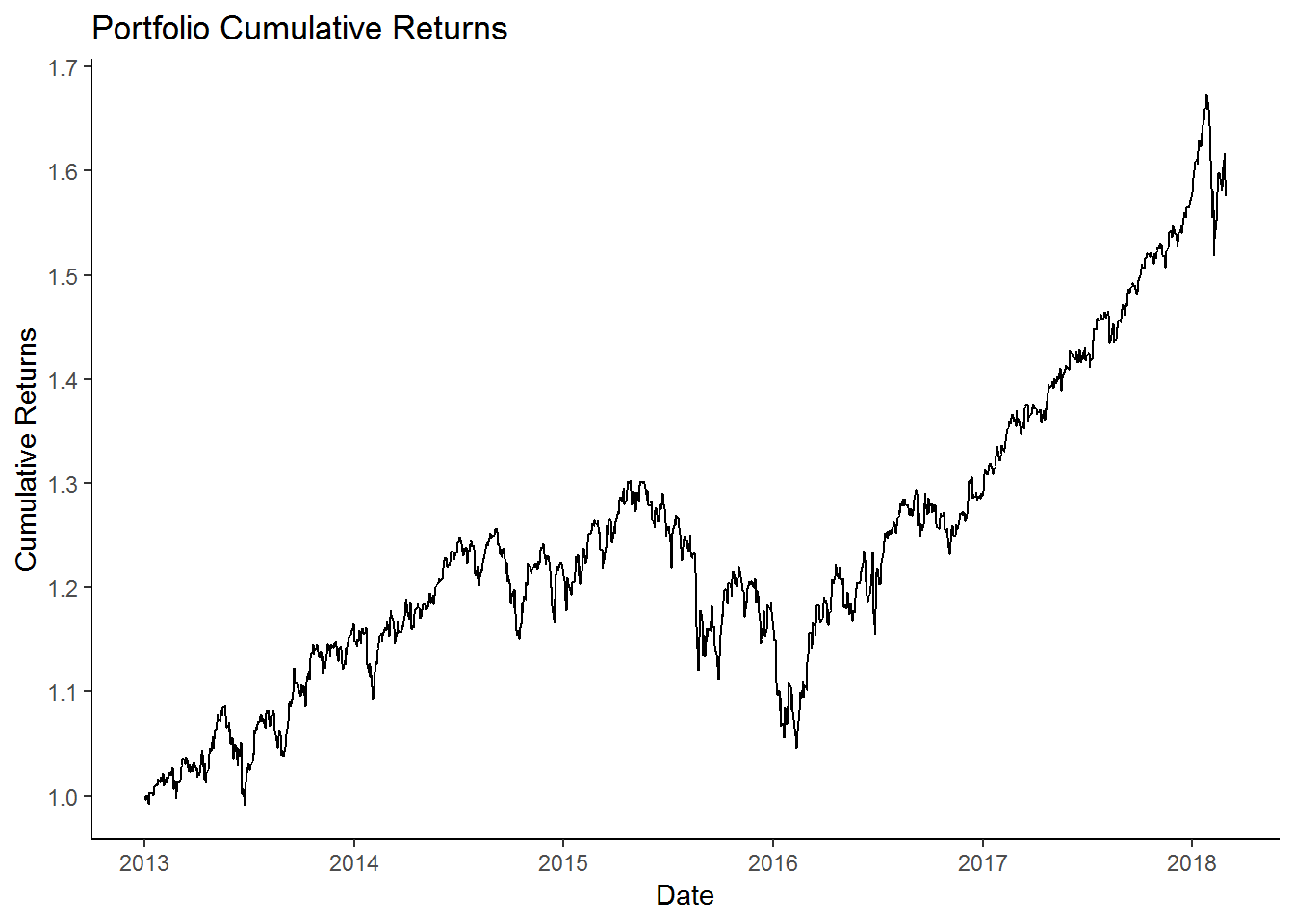

We will post the entire code here.

library(tidyquant)

# Asset tickers

tickers = c('BND', 'VB', 'VEA', 'VOO', 'VWO')

# Asset weights

wts = c(0.1,0.2,0.25,0.25,0.2)

price_data <- tq_get(tickers,
                     from = '2013-01-01',
                     to = '2018-03-01',
                     get = 'stock.prices')

ret_data <- price_data %>%
  group_by(symbol) %>%
  tq_transmute(select = adjusted,
               mutate_fun = periodReturn,
               period = "daily",
               col_rename = "ret")

wts_tbl <- tibble(symbol = tickers,
                  wts = wts)
ret_data <- left_join(ret_data,wts_tbl, by = 'symbol')

ret_data <- ret_data %>%
  mutate(wt_return = wts * ret)

port_ret <- ret_data %>%
  group_by(date) %>%
  summarise(port_ret = sum(wt_return))

port_cumulative_ret <- port_ret %>%
  mutate(cr = cumprod(1 + port_ret))

But there is a simpler code if we use the tidyquant function. We will demonstrate how to use to tidyquant to calculate cumulative portfolio returns.

port_ret_tidyquant <- ret_data %>%
  tq_portfolio(assets_col = symbol,
               returns_col = ret,
               weights = wts,
               col_rename = 'port_ret',
               geometric = FALSE)

port_cumulative_ret_tidyquant <- port_ret_tidyquant %>%
  mutate(cr = cumprod(1 + port_ret))

As we can see that the above code is much shorter than the previous code. We can compare the two portfolio calculations.

port_cumulative_ret %>%
  mutate(port_ret_tidyquant = port_cumulative_ret_tidyquant$cr) %>%
  select(-port_ret) %>%
  rename(long_method = cr) %>%
  gather(long_method,port_ret_tidyquant,
         key = port_method,
         value = cr) %>%
  ggplot(aes(x = date, y = cr, color = port_method)) +
  geom_line() +
  labs(x = 'Date',
       y = 'Cumulative Returns',
       title = 'Portfolio Cumulative Returns') +
  theme_classic() +
  scale_y_continuous(breaks = seq(1,2,0.1)) +
  scale_x_date(date_breaks = 'year',
               date_labels = '%Y')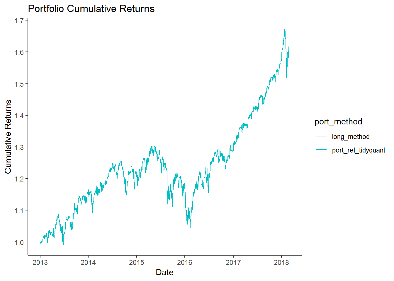

We can see that both line overlap each other and the returns are the same. So in the future its best to use the shorter tq_portfolio() method.