How to calculate portfolio statistics in R

In this post we will calculate the following portfolio statistics using R.

Portfolio average returns
Portfolio standard deviation
Portfolio Sharpe ratio

As usual we will start with loading our libraries.

library(tidyquant)
library(timetk)

We will use the same assets from the last post to build our portfolio.

# Create the tickers and weights vector

tickers = c('BND', 'VB', 'VEA', 'VOO', 'VWO')

wts = c(0.1,0.2,0.25,0.25,0.2)

Next lets download the price data from yahoo finance.

price_data <- tq_get(tickers,
                     from = '2013-01-01',
                     to = '2018-03-01',
                     get = 'stock.prices')

Next we will calculate the daily returns for our assets.

ret_data <- price_data %>%
  group_by(symbol) %>%
  tq_transmute(select = adjusted,
               mutate_fun = periodReturn,
               period = "daily",
               col_rename = "ret")

We will use the tq_portfolio package to quickly calculate the portfolio returns.

port_ret <- ret_data %>%
  tq_portfolio(assets_col = symbol,
               returns_col = ret,
               weights = wts,
               col_rename = 'port_ret',
               geometric = FALSE)

Lets look at the total cumulative returns for our portfolio.

port_ret %>%
  mutate(cr = cumprod(1 + port_ret)) %>%
  ggplot(aes(x = date, y = cr)) +
  geom_line() +
  labs(x = 'Date',
       y = 'Cumulative Returns',
       title = 'Portfolio Cumulative Returns') +
  theme_bw() +
  scale_y_continuous(breaks = seq(1,2,0.1)) +
  scale_x_date(date_breaks = 'year',
               date_labels = '%Y')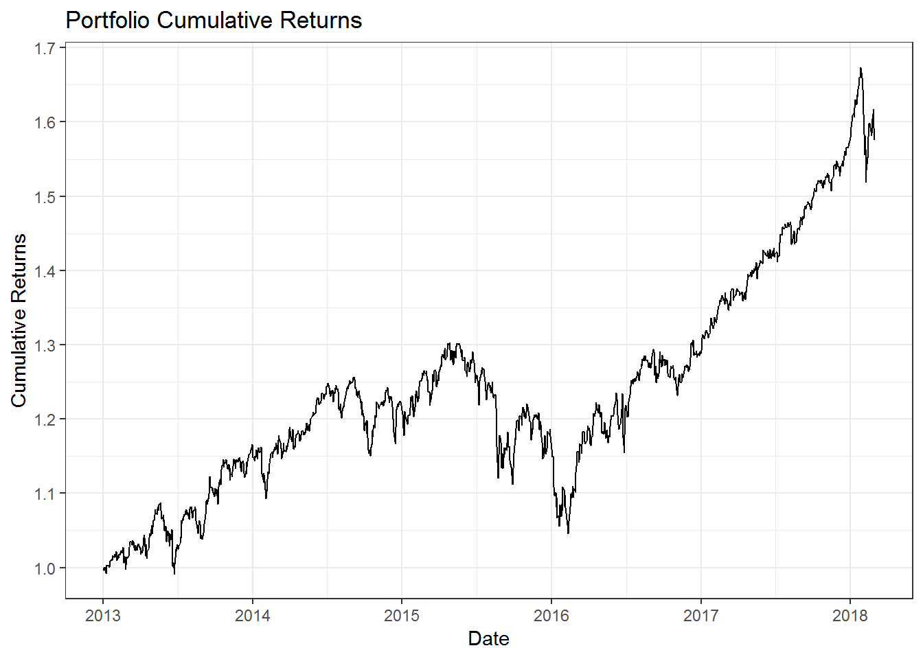

Now lets begin by calculating the average annual portfolio returns.

average_annual_port_ret <- port_ret %>%
  tq_performance(Ra = port_ret,
                 performance_fun = Return.annualized)

cat("The average annual portfolio returns is ", round((average_annual_port_ret[[1]] * 100),2),"%", sep = "")

## The average annual portfolio returns is 9.22%

Next we will calculate the portfolio standard deviation or volatility. There are two methods to do this. We will first calculate this manually. For that we need to calculate the daily portfolio volatility.

daily_port_sd <- sd(port_ret$port_ret)

cat("The daily portfolio volatility is", round((daily_port_sd),4))

## The daily portfolio volatility is 0.0076

Now we need to annualize this to find the annual volatility.

annual_port_sd <- daily_port_sd * sqrt(252)

cat("The annual portfolio volatility is", round((annual_port_sd),4))

## The annual portfolio volatility is 0.1204

We can use the built in formula to calculate this as well, but to use that we need to convert our data into an xts format. We can do that as shown below.

annual_port_sd_xts <- StdDev.annualized(tk_xts(port_ret, silent = TRUE))

cat("The annual portfolio volatility using the xts method is", round((annual_port_sd_xts),4))

## The annual portfolio volatility using the xts method is 0.1204

We can see that we get the same answer. Use whatever method you find easier.

Next we will find the portfolio’s Sharpe ratio. We will first calculate it manually and then we will use the built in formula.

sharpe_ratio_manually <- average_annual_port_ret$AnnualizedReturn / annual_port_sd

cat("The annual portfolio sharpe ratio calculated manually is", round((sharpe_ratio_manually),4))

## The annual portfolio sharpe ratio calculated manually is 0.7658

If Risk free interest rate is 4% (as it was pre 2008 crisis), then we get the Sharpe ratio as follows.

sharpe_ratio_manually_rf_4 <- (average_annual_port_ret$AnnualizedReturn - 0.04) / annual_port_sd

cat("The annual portfolio sharpe ratio calculated manually when risk free interest rate is at 4% is", round((sharpe_ratio_manually_rf_4),4))

## The annual portfolio sharpe ratio calculated manually when risk free interest rate is at 4% is 0.4337

We could do this using the tq_performance function.

sharpe_ratio <- port_ret %>%
  tq_performance(Ra = port_ret,
                 performance_fun = SharpeRatio.annualized) %>%
  .[[1]]

cat("The annual portfolio sharpe ratio calculated using the tq_performance function is", round((sharpe_ratio),4))

## The annual portfolio sharpe ratio calculated using the tq_performance function is 0.7658

We can also change the risk free rate to 4%.

sharpe_ratio_rf_4 <- port_ret %>%
  tq_performance(Ra = port_ret,
                 performance_fun = SharpeRatio.annualized,
                 Rf = 0.04/252) %>%
  .[[1]]

cat("The annual portfolio sharpe ratio calculated using the tq_performance function when Rf is 45 is", round((sharpe_ratio_rf_4),4))

## The annual portfolio sharpe ratio calculated using the tq_performance function when Rf is 45 is 0.4103

This is slightly different that our manually calculated number. This is due to the tq_performance function calculating the daily excess returns and then annualizing it. This causes the slight difference between our manual calculation, which ignored the daily excess returns.